Blog post six

Our group has determined the the metric in which we will use to compare the OECD and HIPC countries. We will track GDP per capita over time and study how certain factors correspond to the growth of GDP per Capita. The factors of study are isted below.

1. education expenditure
2. gross savings
3. compensation for employees
4. tax revenue % of GDP
5. GDP Growth (Might not be neccessary given what we’re using to measure economic development)
6. FDI
7. Monetary Sector Credit to Private Sector as % of GDP
8. Unemployment rate

This week we studied how these covariates relate to the rise of GDP per capita in HIPC across the world. Firstly we will study Monetary Sector Credit to Private Sector as % of GDP and how it relates to gdp per capita.

library(ggplot2)
data.in <- read.csv(file.choose())
head(data.in)

##      MSC_70    FDI_70      GDP_70  X X.1    EE_70 Year_70    GDPPC
## 1  9.672431 0.9119564 1.49480e+11 NA  NA 3.082898    1970 719.6410
## 2 10.092079 0.6469092 1.55825e+11 NA  NA 3.269036    1971 730.6380
## 3 10.680662 0.7033483 1.58462e+11 NA  NA 3.484333    1972 723.5575
## 4 11.255663 0.7616990 1.63032e+11 NA  NA 3.479373    1973 724.8922
## 5 12.612460 0.7038800 1.72314e+11 NA  NA 3.276370    1974 746.0455
## 6 13.973724 0.6303407 1.75802e+11 NA  NA 3.470933    1975 741.1724

plot(data.in$MSC_70, data.in$GDPPC)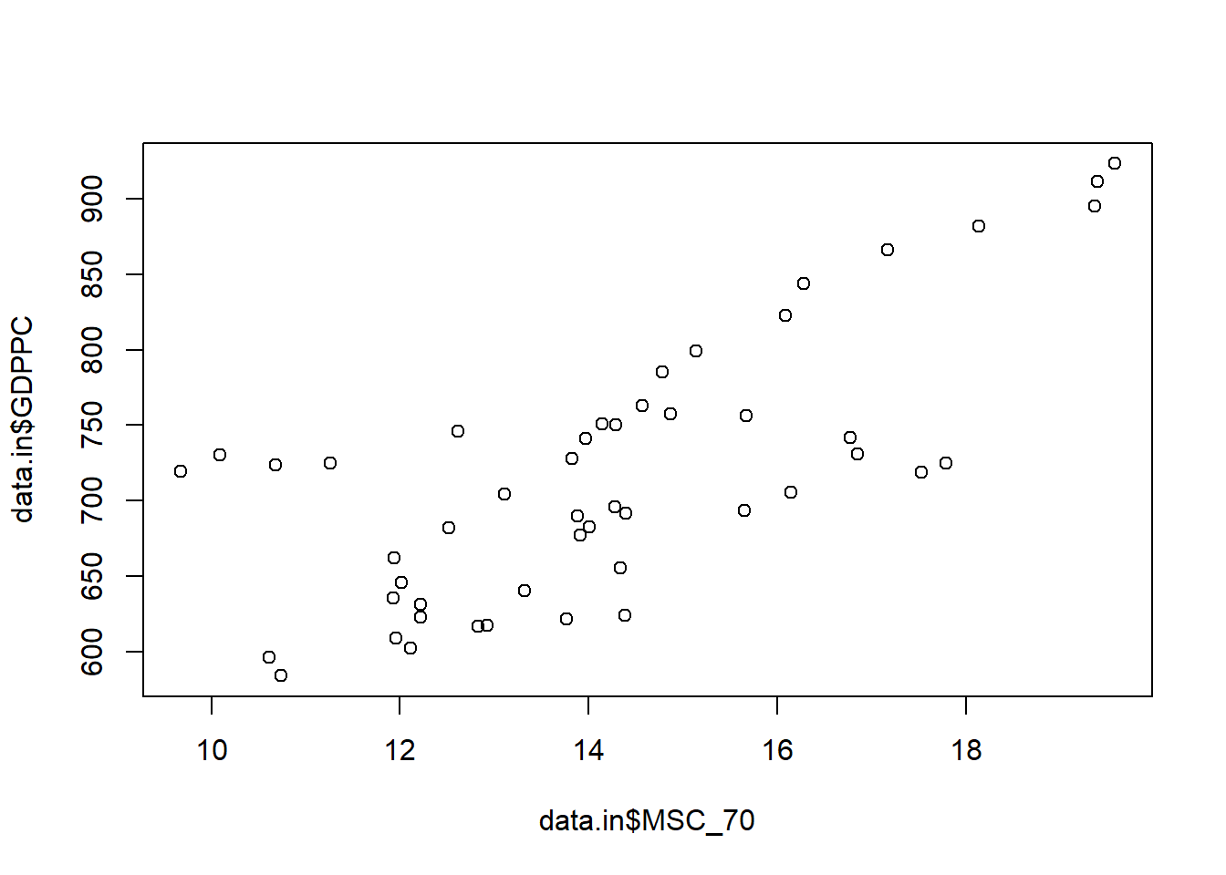

MSC <- lm(data.in$GDPPC ~ data.in$MSC_70)
summary(MSC)

## 
## Call:
## lm(formula = data.in$GDPPC ~ data.in$MSC_70)
## 
## Residuals:
##    Min     1Q Median     3Q    Max 
## -97.37 -50.57 -15.54  53.83 118.06 
## 
## Coefficients:
##                Estimate Std. Error t value Pr(>|t|)    
## (Intercept)     356.192     50.105   7.109 5.59e-09 ***
## data.in$MSC_70   25.404      3.478   7.304 2.83e-09 ***
## ---
## Signif. codes:  0 '***' 0.001 '**' 0.01 '*' 0.05 '.' 0.1 ' ' 1
## 
## Residual standard error: 59.19 on 47 degrees of freedom
## Multiple R-squared:  0.5316, Adjusted R-squared:  0.5217 
## F-statistic: 53.35 on 1 and 47 DF,  p-value: 2.833e-09

equation1=function(x){coef(MSC)[2]*x+coef(MSC)[1]}
MSCp <- ggplot(data.in ,aes(y=GDPPC,x=MSC_70,color="blue"))+
  geom_point()+
  stat_function(fun=equation1,geom="line",color=scales::hue_pal()(2)[1]) +
  xlab("MSC")+
  ylab("GDP per Capita")+
  ggtitle("How does MSC relate to GDP per Capita")
MSCp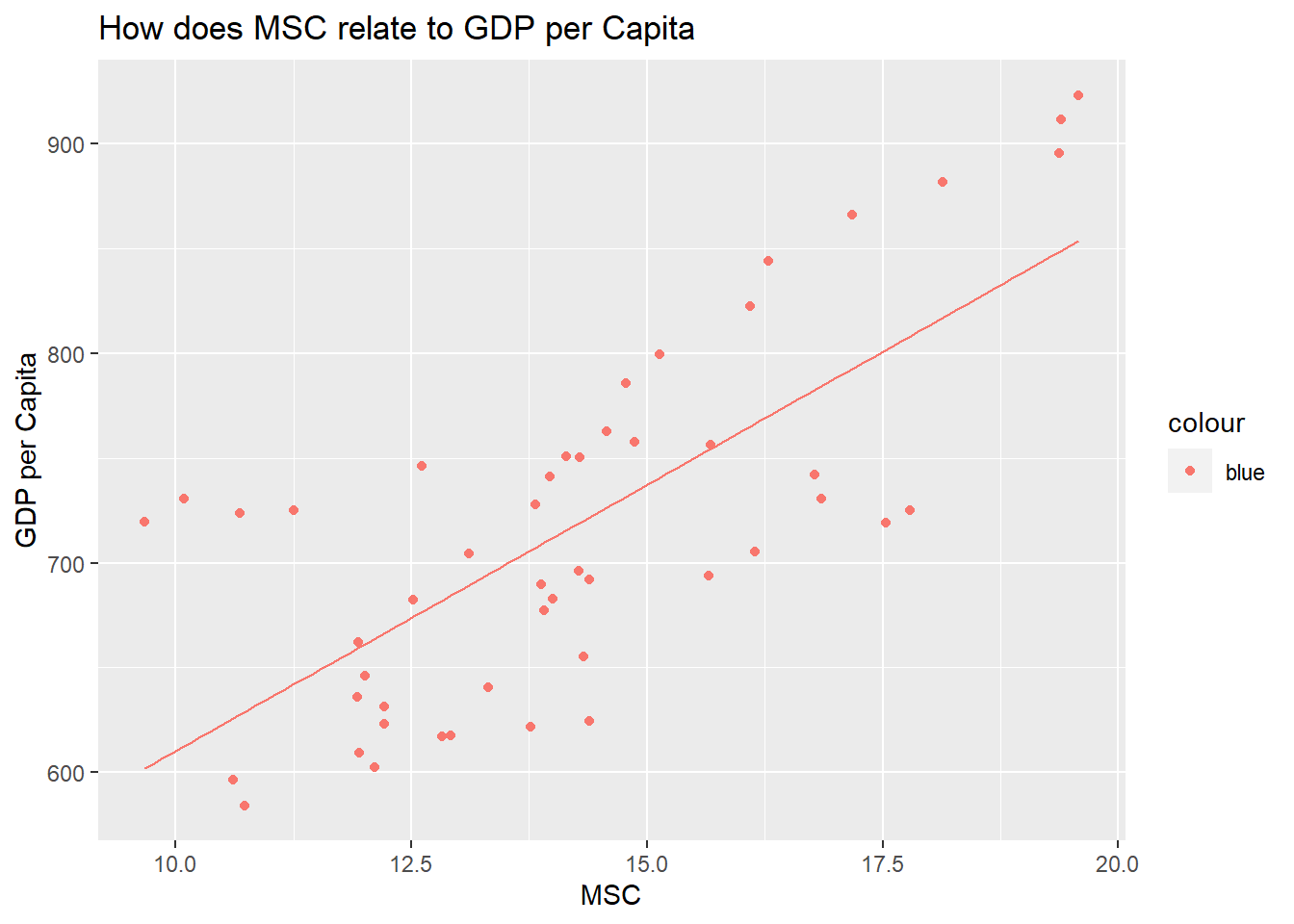

We should conclude from this model that MSC is related to the growth of a nation’s GDP percapita. In this case specifically, it is correlated to growth in HIPC countries. The actor’s coefficient is highly significant with a test statistic of 7.304 and has a corresponding p-value of <.00001.

We will repeat this process with another covariate for this blog post.

Next we will examine FDi

plot(data.in$FDI_70, data.in$GDPPC)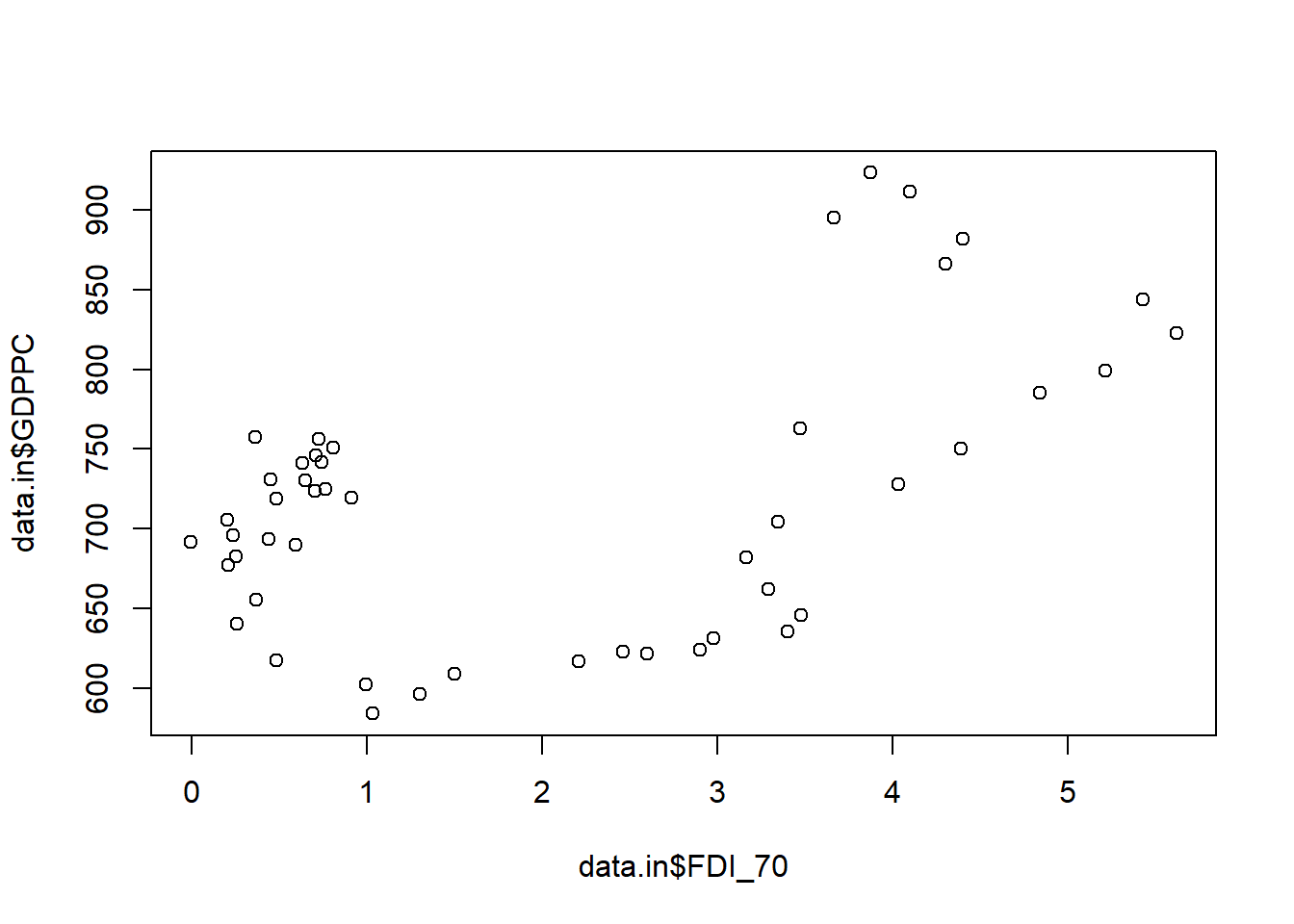

FDINORM <- lm(data.in$GDPPC ~ data.in$FDI_70)
summary(FDINORM)

## 
## Call:
## lm(formula = data.in$GDPPC ~ data.in$FDI_70)
## 
## Residuals:
##     Min      1Q  Median      3Q     Max 
## -113.34  -62.60   11.94   46.93  162.82 
## 
## Coefficients:
##                Estimate Std. Error t value Pr(>|t|)    
## (Intercept)      668.89      16.87  39.650  < 2e-16 ***
## data.in$FDI_70    23.61       6.35   3.719 0.000533 ***
## ---
## Signif. codes:  0 '***' 0.001 '**' 0.01 '*' 0.05 '.' 0.1 ' ' 1
## 
## Residual standard error: 76.03 on 47 degrees of freedom
## Multiple R-squared:  0.2274, Adjusted R-squared:  0.2109 
## F-statistic: 13.83 on 1 and 47 DF,  p-value: 0.0005327

sqrFDI <- (data.in$FDI_70)^2
FDI <- lm(data.in$GDPPC ~ data.in$FDI_70 + sqrFDI)
summary(FDI)

## 
## Call:
## lm(formula = data.in$GDPPC ~ data.in$FDI_70 + sqrFDI)
## 
## Residuals:
##    Min     1Q Median     3Q    Max 
## -94.08 -59.21 -19.49  42.77 180.69 
## 
## Coefficients:
##                Estimate Std. Error t value Pr(>|t|)    
## (Intercept)     713.532     20.780  34.337  < 2e-16 ***
## data.in$FDI_70  -49.132     23.434  -2.097  0.04156 *  
## sqrFDI           14.628      4.565   3.204  0.00246 ** 
## ---
## Signif. codes:  0 '***' 0.001 '**' 0.01 '*' 0.05 '.' 0.1 ' ' 1
## 
## Residual standard error: 69.49 on 46 degrees of freedom
## Multiple R-squared:  0.3683, Adjusted R-squared:  0.3409 
## F-statistic: 13.41 on 2 and 46 DF,  p-value: 2.578e-05

data.in$pred.fdi  <- predict.lm(FDI) 
length(data.in$GDPPC)

## [1] 49

length(data.in$FDI_70)

## [1] 49

FDIp <- ggplot(data.in, aes(y=GDPPC,x=pred.fdi ,color="blue"))+
  geom_point()+
  geom_smooth(method = "lm", se = FALSE)+
  xlab("FDI")+
  ylab("GDP per Capita")+
  ggtitle("How does FDI relate to GDP per Capita")
FDIp

## `geom_smooth()` using formula 'y ~ x'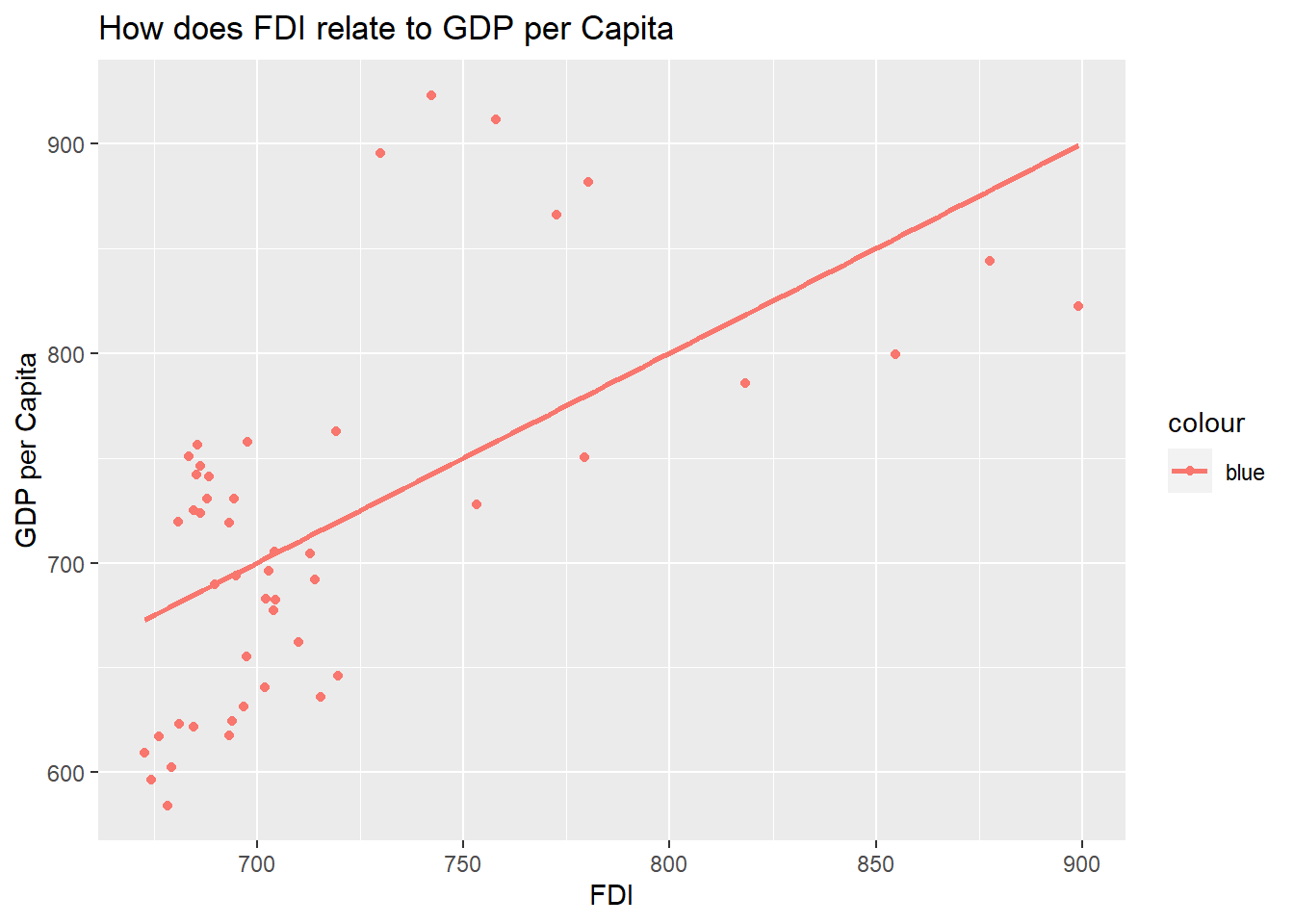

While the summary of the data is indicating that FDI has a positive linear relationship with GDP per Capita, I belive a linear trend may not be the most efficient at modeling the data’s relationship. In future analysis we will adjust and transfrom the data to fit a better model. We attempted to fit the model with a quadratic term however there still seems to be issues with the model fit with a high cluster in the lesser values of FDI.

We will continue with this data analysis to inform the creation of a multivariate linear model to predict GDP per Capita in HIPC countries. We will repeat the process for OECD countries and compare the relationships between these metrics and more developed nations.