library(dplyr)##
## Attaching package: 'dplyr'## The following objects are masked from 'package:stats':
##
## filter, lag## The following objects are masked from 'package:base':
##
## intersect, setdiff, setequal, unionlibrary(ggplot2)Loading the Data
After our recent blog posts, we have a better understanding of the metrics and relationships between HIPC and OECD member countries. Building on those, we have decided to narrow our focus on HIPC countries and begin building a model to understand the factors that lead to gdp growth.
For this intial model building exercise we have selected:
- Adjusted net enrollment rate, primary (% of primary school age children)
- Access to electricity (% of population)
- Inflation, consumer prices (annual %)
To predict: GDP per capita (constant 2010 US$)
We believe these factors provided in the WDI database give a reasonable picture of economic growth of a country that should impact the GDP of a growing country.
data <- read.csv('~/Documents/courses/ma415/final-project-data/blog-4-data-final.csv')full_subset <- data %>% select(X2003..YR2003.:X2018..YR2018.)
series_name = data$Series.NameWe use a subset of the data were all factors are available over a period of almost two decades. We continue to clean and prepare the data for a simple multivariable regression model.
access_elec   <- as.numeric(as.character(full_subset[1,]))

# We remove the following as they are redudant in our model
#com_edu       <- as.numeric(as.character(full_subset[3,]))

primary_enrol <- as.numeric(as.character(full_subset[2,]))
gdp           <- as.numeric(as.character(full_subset[4,]))
inflation     <- as.numeric(as.character(full_subset[5,]))

regression_data <- data_frame(access_elec=access_elec, primary_enrol=primary_enrol, inflation=inflation, gdp=gdp)
## Warning: `data_frame()` is deprecated as of tibble 1.1.0.
## Please use `tibble()` instead.
## This warning is displayed once every 8 hours.
## Call `lifecycle::last_warnings()` to see where this warning was generated.head(regression_data)## # A tibble: 6 x 4
## access_elec primary_enrol inflation gdp
## <dbl> <dbl> <dbl> <dbl>
## 1 23.6 63.0 5.30 646.
## 2 24.3 65.6 4.57 662.
## 3 22.3 68.2 8.45 682.
## 4 25.8 70.7 6.78 704.
## 5 34.4 72.8 7.60 728.
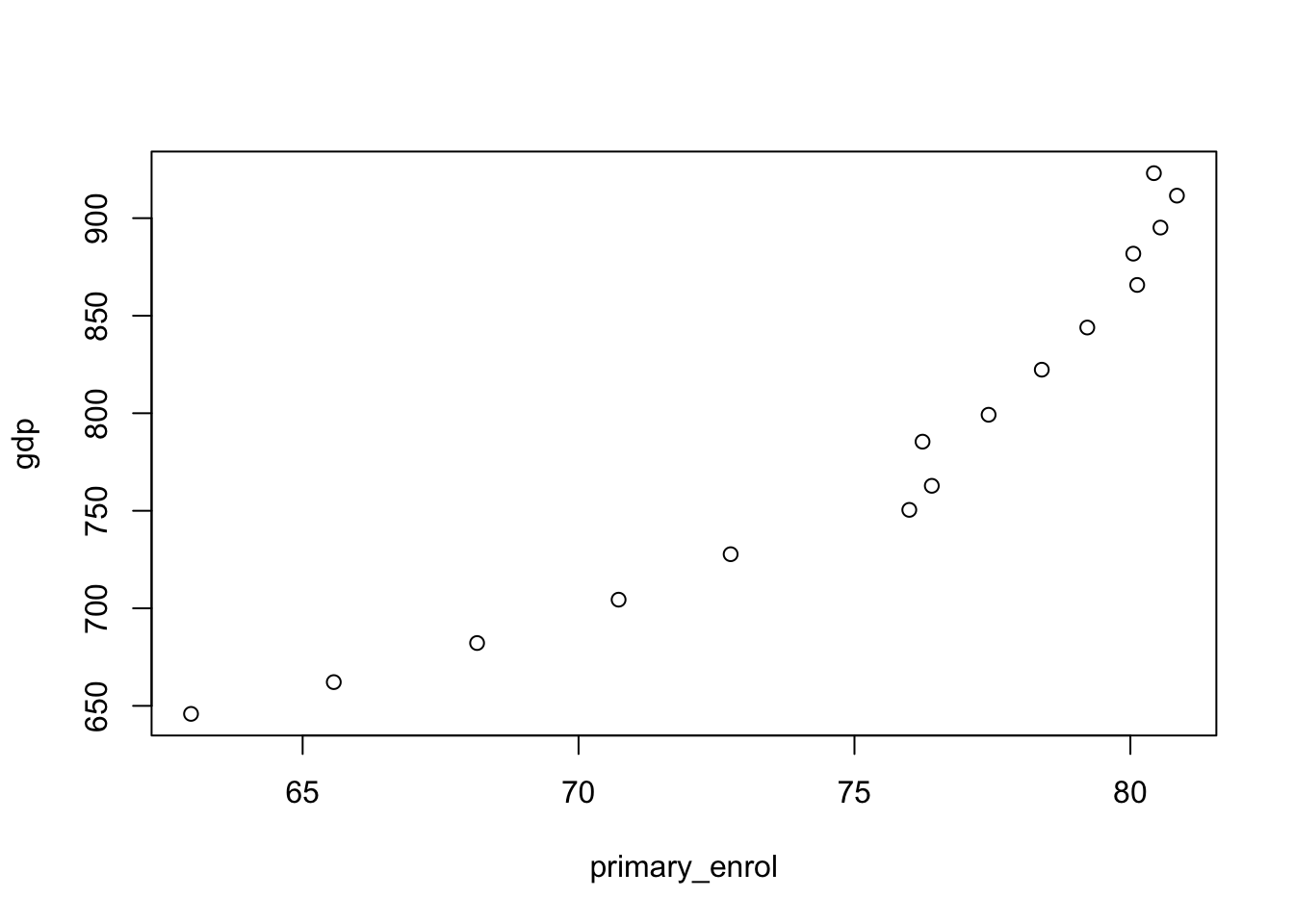
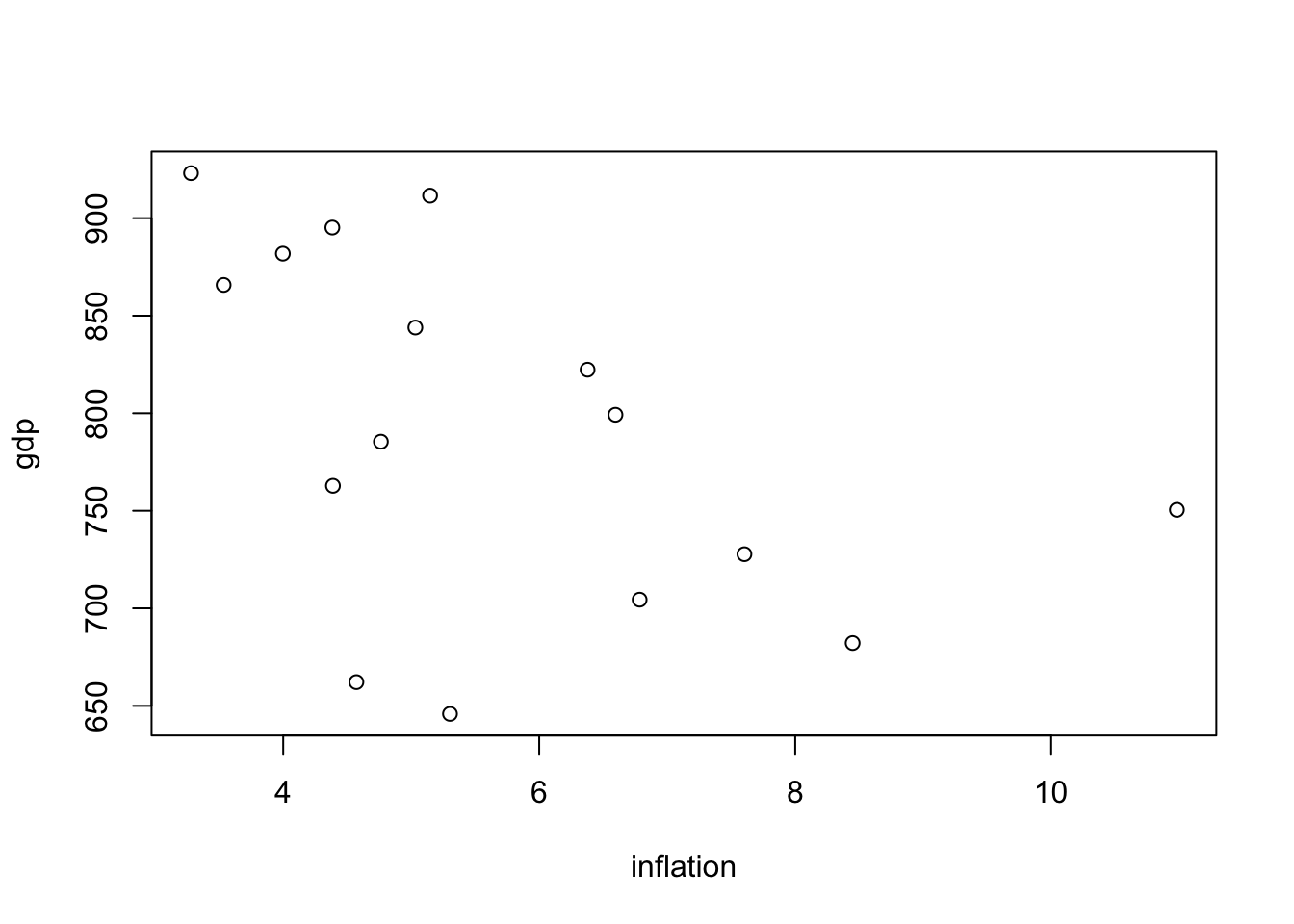
## 6 28.0 76.0 11.0 750.Before fitting our model we inspect the plots of each individual variable and observe a generally linear trends:
plot(gdp ~ access_elec + primary_enrol + inflation, regression_data)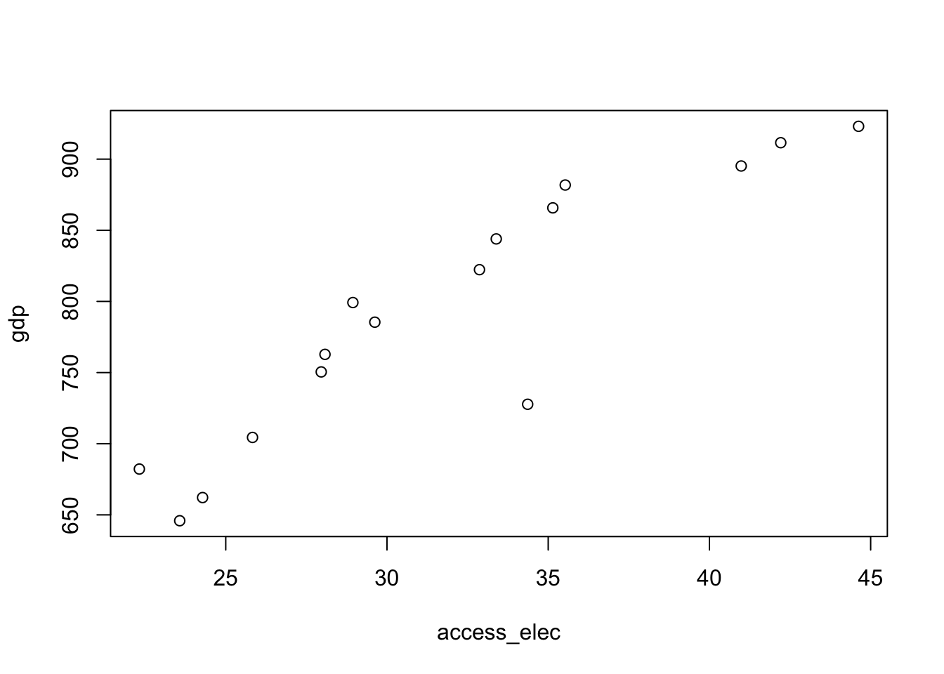
Fitting the Model
fit <- lm(gdp ~ access_elec + primary_enrol + inflation, data = regression_data)
summary(fit) # show results
##
## Call:
## lm(formula = gdp ~ access_elec + primary_enrol + inflation, data = regression_data)
##
## Residuals:
## Min 1Q Median 3Q Max
## -39.268 -4.092 1.968 8.525 23.707
##
## Coefficients:
## Estimate Std. Error t value Pr(>|t|)
## (Intercept) -65.367 77.150 -0.847 0.41342
## access_elec 4.873 1.230 3.962 0.00189 **
## primary_enrol 9.756 1.354 7.204 1.08e-05 ***
## inflation -5.906 2.566 -2.302 0.04005 *
## ---
## Signif. codes: 0 '***' 0.001 '**' 0.01 '*' 0.05 '.' 0.1 ' ' 1
##
## Residual standard error: 17.68 on 12 degrees of freedom
## Multiple R-squared: 0.9697, Adjusted R-squared: 0.9622
## F-statistic: 128.2 on 3 and 12 DF, p-value: 2.225e-09After fitting the model we can see form the incredibly high R^squared value that this model captures the data very well. We also observe that all covariates are individually significant at the 95% level. Note that the coefficient estimates also follow intuition as education and electricity access increases so does economic activity measured as GDP. Inflation as is observed to have a negative impact on GDP so we capture postive and negative relationships in out data.
We believe this is a good beginning into the modeling we can do on this database and will be continuing to explore more complex and interesting relationships in the data.