library(tidyverse)## -- Attaching packages --------------------------------------- tidyverse 1.3.0 --## v ggplot2 3.3.3 v purrr 0.3.4
## v tibble 3.0.5 v dplyr 1.0.3
## v tidyr 1.1.2 v stringr 1.4.0
## v readr 1.4.0 v forcats 0.5.0## -- Conflicts ------------------------------------------ tidyverse_conflicts() --
## x dplyr::filter() masks stats::filter()
## x dplyr::lag() masks stats::lag()Raw_data <- readxl::read_xlsx("~/MA415 project/GDP_TRADE (2).xlsx")
GDP_TRADE <- Raw_data %>% filter(`Indicator Name` == "GDP (constant 2010 US$)"|`Indicator Name` == "Exports of goods and services (% of GDP)"|`Indicator Name` =="Imports of goods and services (% of GDP)"|`Indicator Name` == "GDP growth (annual %)") %>%
pivot_longer(cols=!`Country Name`&!`Country Code`&!`Indicator Name`&!`Indicator Code`,names_to="year",values_to="Indicator Value")%>%pivot_wider(id_cols=c(`Country Name`,year),names_from=`Indicator Name`,values_from=`Indicator Value`)%>%mutate("Net Trade (constant 2010 US$)" = (`Exports of goods and services (% of GDP)`-`Imports of goods and services (% of GDP)`)*`GDP (constant 2010 US$)`, "Exports of goods and services (constant 2010 US$)" = `Exports of goods and services (% of GDP)` *`GDP (constant 2010 US$)`,"Imports of goods and services (constant 2010 US$)" = `Imports of goods and services (% of GDP)` * `GDP (constant 2010 US$)`) %>%pivot_longer(cols = !`Country Name`&!`year`, names_to="Indicator",values_to="Value")
GDP_CONSTANT_TRADE <- GDP_TRADE%>%filter(Indicator == "GDP (constant 2010 US$)"| Indicator == "Exports of goods and services (constant 2010 US$)"| Indicator == "Imports of goods and services (constant 2010 US$)")
GDP_CONSTANT_TRADE_NET <- GDP_TRADE%>%filter(Indicator == "Net Trade (constant 2010 US$)"| Indicator == "GDP (constant 2010 US$)")
GDP_PROP_TRADE_NET <- GDP_TRADE%>%filter(Indicator == "Net Trade (constant 2010 US$)"|Indicator == "GDP (constant 2010 US$)")First, we try to examine the trade between the country of OECD members and those HIPC countries by analyzing the their Exports and Imports of goods and service separately. As the plot shown below, the “Heavily INdebted Poor Countries”(HPC) tends to have lower GDP and Exports/Imports, on the other hand, the OECD members have much more Imports/Exports, which also significantly outweigh its GDP value. However, this plot doest not tell the story about the relationship of the net trade and the countries’ GDP.
GDP_CONSTANT_TRADE %>% ggplot() + geom_line(aes(x = year, y = `Value`, color = `Indicator`, group = Indicator)) + facet_grid(`Country Name` ~.) + xlab("YEAR") + ylab("Value(constant 2010 US$)")+scale_x_discrete(guide = guide_axis(n.dodge=3))## Warning: Removed 13 row(s) containing missing values (geom_path).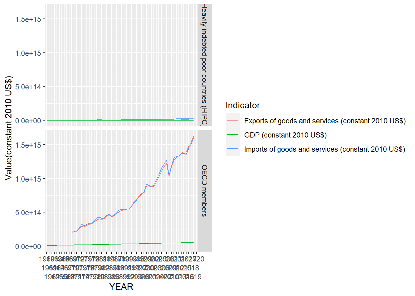 As shown by the chart below, OECD members and HPCs’ net trade are always below their GDP. However, the OECD members, clearly, has significant more variance on net trade value and shows a increasing trend of net trade over the years.
GDP_CONSTANT_TRADE_NET %>% ggplot() + geom_line(aes(x = year, y = `Value`, color = `Indicator`, group = Indicator)) + facet_grid(`Country Name` ~.) + xlab("YEAR") + ylab("Value(constant 2010 US$)")+scale_x_discrete(guide = guide_axis(n.dodge=3))## Warning: Removed 7 row(s) containing missing values (geom_path).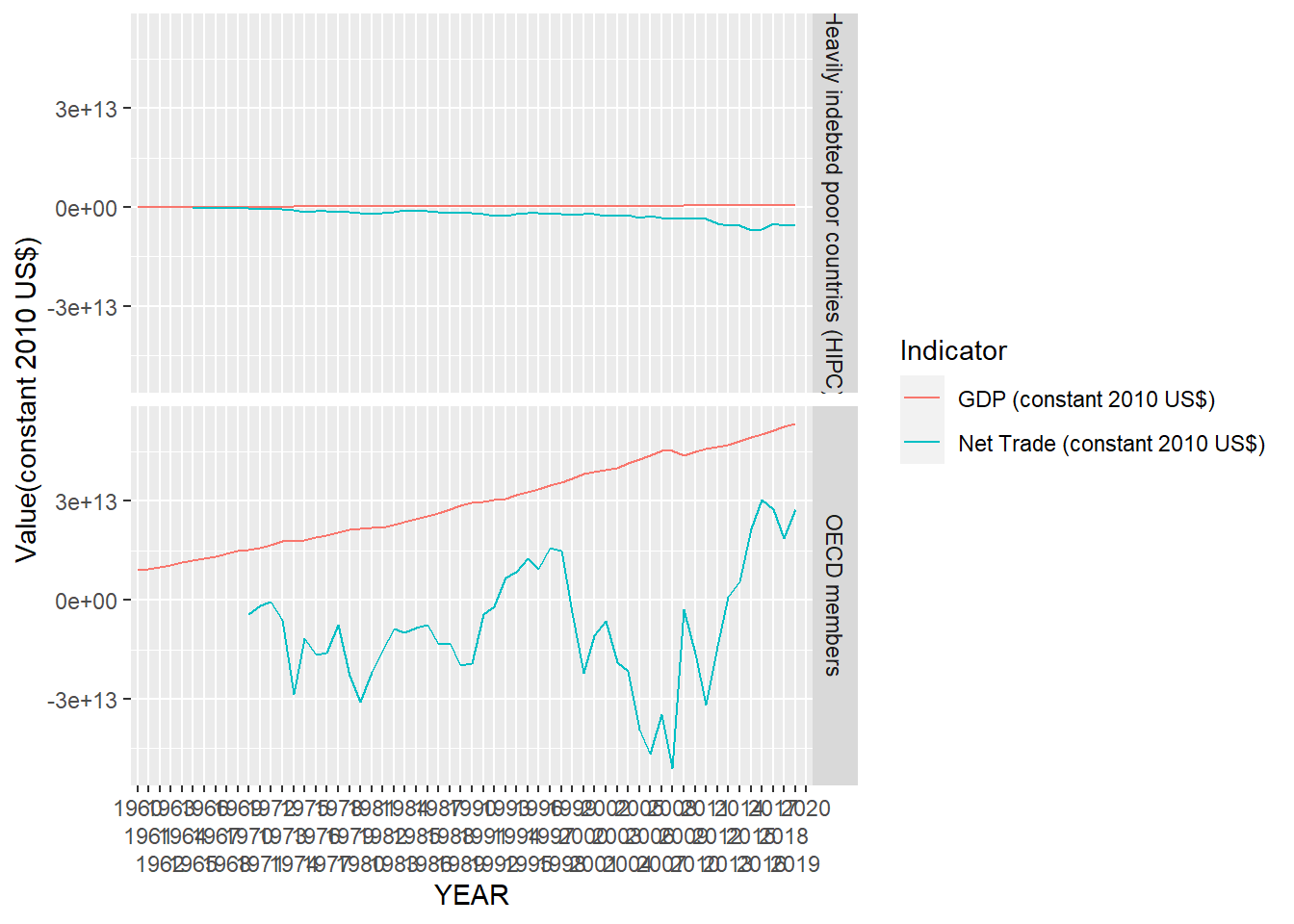 To further investigate whether how much value of Net Trade contribute to the OECD/HPC’s GDP, we plot the graph as shown below. The GDP of HPC are much relied on the Net trade comparing to the OECD members. Also, the the value of the net trade of HPC has less variance comparing to the OECD members.
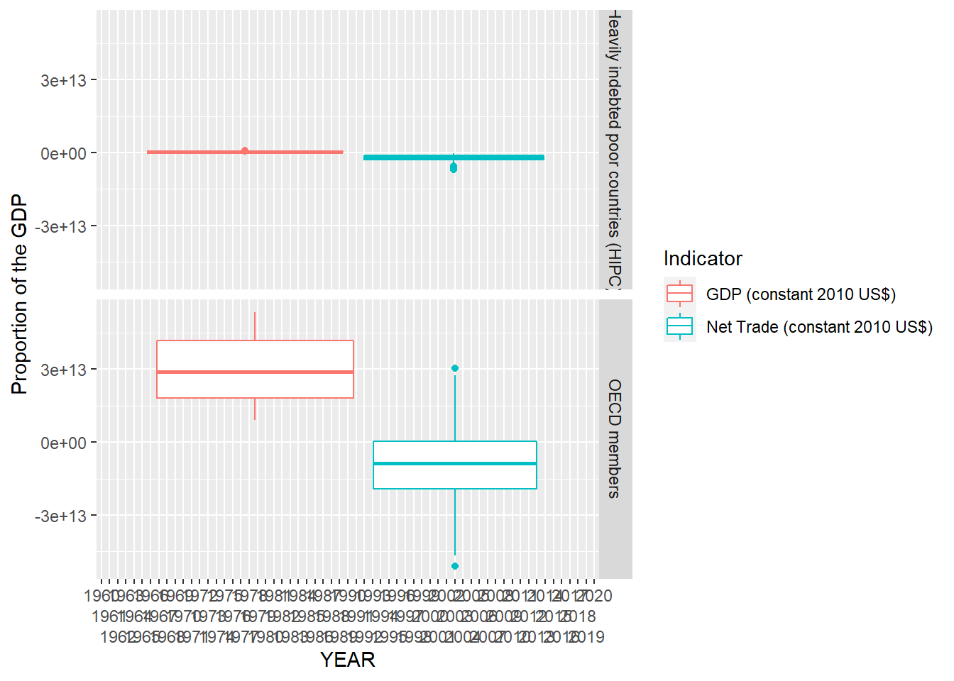
GDP_PROP_TRADE_NET %>% ggplot() + geom_boxplot(aes(x = year, y = `Value`, color = `Indicator`, group = Indicator))+ facet_grid(`Country Name` ~.) + xlab("YEAR") + ylab("Proportion of the GDP")+scale_x_discrete(guide = guide_axis(n.dodge=3))## Warning: Removed 19 rows containing non-finite values (stat_boxplot).