
WDI Variable Analysis
For this variable analysis we focus on the World Development Indicator (WDI) dataset that acts our main datasource. To begin our analysis we have selected to following variables as potential coviariates after our thorough data clean detailed earlier.
- GDP per capita (current US$)
- Gross domestic savings (current US$)
- GDP growth (annual %)
- Foreign direct investment, net inflows (BoP, current US$)
- Foreign direct investment, net outflows (BoP, current US$)
- Unemployment, male (% of male labor force) (modeled ILO estimate)
Notes on this dataset:
- Unemployment data for females was scarce and difficult to use for analysis. Therefore, we decided to use solely male data.
However, we don’t want to just understand what factors may play a role in GDP growth for a country. We want to further understand the differences between developing (HIPC) and developed (OECD) countries. For this, the WDI dataset provides aggregate country information based on these criterion: the Heavily Indebted PoorCountry (HIDPC) aggregate, and the Organisation for Economic Co-operation and Development (OECD) aggregate.
To begin our coviariate analysis we look at trends over time:
wdi_vars<-c("Country Name",
            "year",
            "GDP per capita (current US$)",
            "Gross domestic savings (current US$)",
            "GDP growth (annual %)",
            "Foreign direct investment, net inflows (BoP, current US$)",
            "Foreign direct investment, net outflows (BoP, current US$)",
            "Unemployment, male (% of male labor force) (modeled ILO estimate)")

wdi_econi<-select(econi_wide, wdi_vars)

head(wdi_econi)
## # A tibble: 6 x 8
## `Country Name` year `GDP per capita… `Gross domestic… `GDP growth (an…
## <chr> <dbl> <dbl> <dbl> <dbl>
## 1 Heavily indeb… 1991 387. 13895719340. 0.693
## 2 OECD members 1991 17825. 4781817831338. 1.36
## 3 Heavily indeb… 1992 344. 8585509611. -0.581
## 4 OECD members 1992 18997. 5007827253074. 2.04
## 5 Heavily indeb… 1993 343. 10229449325. 0.599
## 6 OECD members 1993 19089. 5041846806737. 1.21
## # … with 3 more variables: `Foreign direct investment, net inflows (BoP,
## # current US$)` <dbl>, `Foreign direct investment, net outflows (BoP, current
## # US$)` <dbl>, `Unemployment, male (% of male labor force) (modeled ILO
## # estimate)` <dbl>Now, let’s begin our data exploration by viewing these trends over time. This will give us an idea of the relationships present before diving into modeling.
#trend over time

par(mfrow=c(1,4))
wdi_econi %>% group_by(`Country Name`) %>%
  ggplot(aes(x=year,
             y=`GDP per capita (current US$)`,
             col=`Country Name`)) +
geom_point() 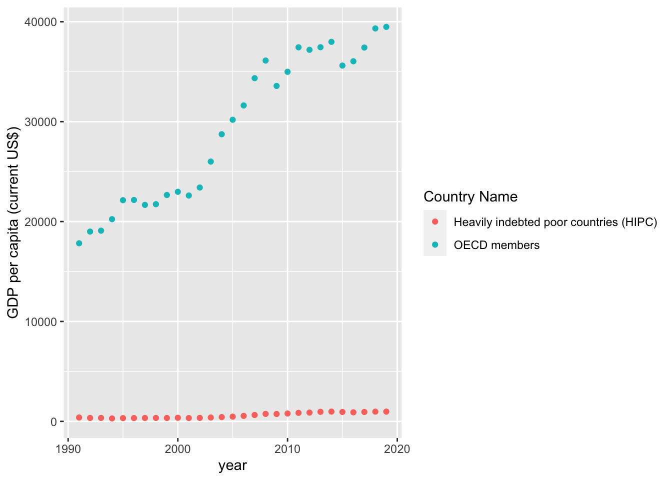
wdi_econi %>% group_by(`Country Name`) %>%
  ggplot(aes(x=year,
             y=`Gross domestic savings (current US$)`,
             col=`Country Name`)) +
geom_point() 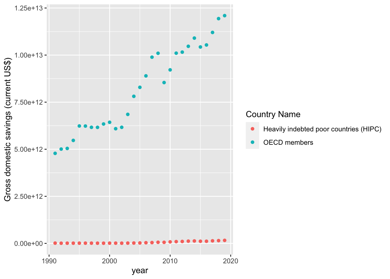
wdi_econi %>% group_by(`Country Name`) %>%
  ggplot(aes(x=year,
             y=`GDP growth (annual %)`,
             col=`Country Name`)) +
geom_point() 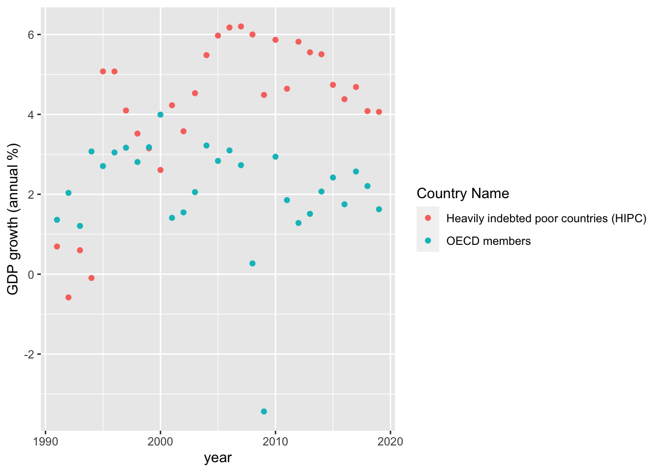
wdi_econi %>% group_by(`Country Name`) %>%
  ggplot(aes(x=year,
             y=`Foreign direct investment, net inflows (BoP, current US$)`,
             col=`Country Name`)) +
geom_point() 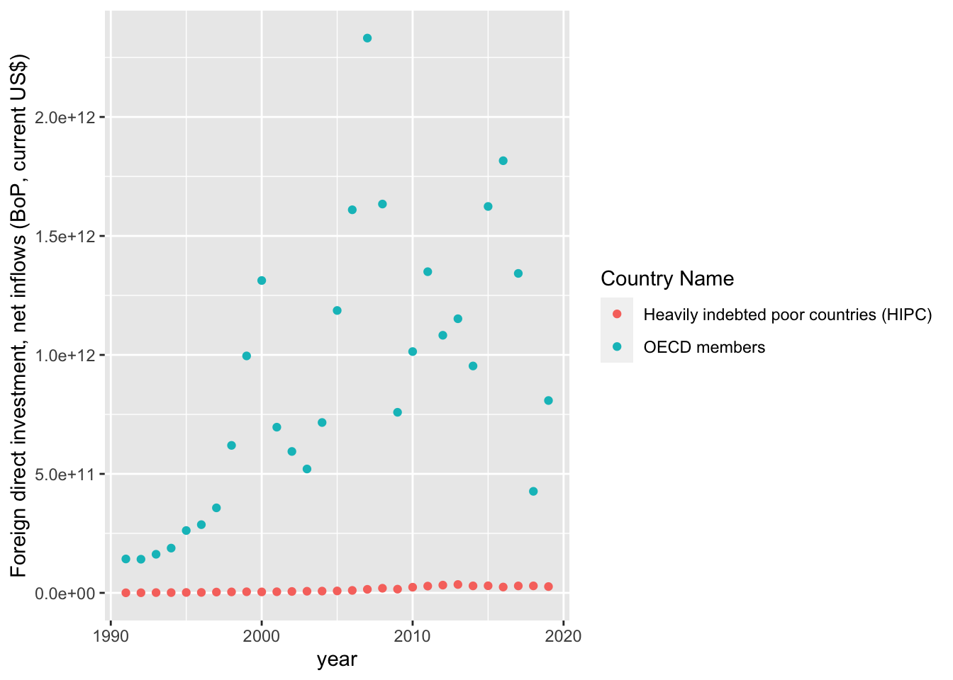
wdi_econi %>% group_by(`Country Name`) %>%
  ggplot(aes(x=year,
             y=`Foreign direct investment, net outflows (BoP, current US$)`,
             col=`Country Name`)) +
geom_point() 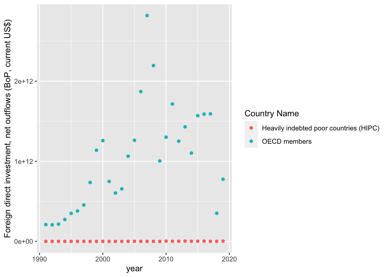
wdi_econi %>% group_by(`Country Name`) %>%
  ggplot(aes(x=year,
             y=`Unemployment, male (% of male labor force) (modeled ILO estimate)`,
             col=`Country Name`)) +
geom_point() 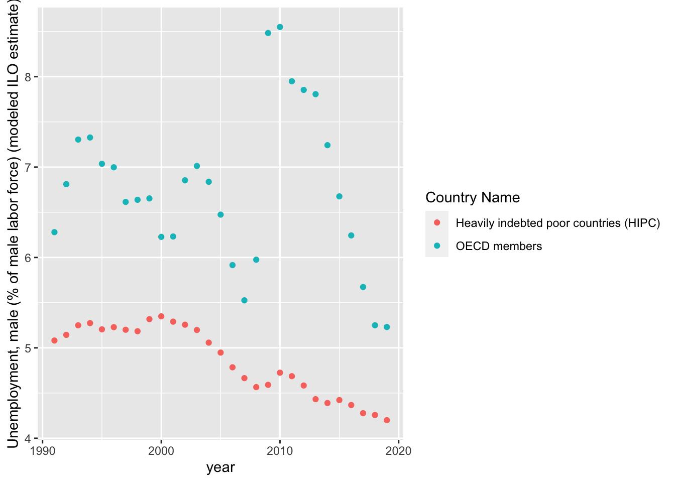
As we can see in the trends there is a massive disparity between HIPC and OECD countries. This difference implies that we should proceed with two seperate models for each group. Additionally, we will have to account for non-linear patterns present in the trends above. In the meantime, let us continue our data exploration with two scatterplots - one for each country group.
HIPC Scatterplot
corr_df <-wdi_econi %>%
filter(`Country Name`=="Heavily indebted poor countries (HIPC)") %>%
select(-year)
ggpairs(corr_df,
progress = F,
lower = list(continuous = wrap("points", alpha = 0.8, size=0.2),
mapping=ggplot2::aes(colour=corr_df$`Country Name`))) +
theme(legend.position = "bottom")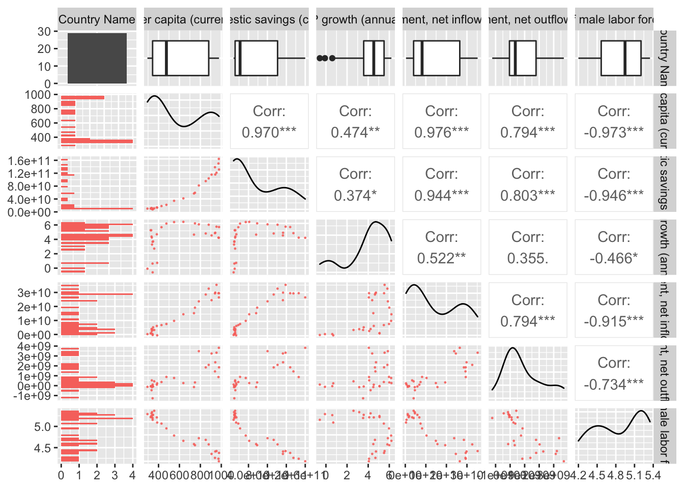 ### OECD Scatterplot
corr_df <-wdi_econi %>% filter(`Country Name`=="OECD members") %>% select(-year)

ggpairs(corr_df,
        progress = F,
        lower = list(continuous = wrap("points", alpha = 0.8, size=0.2),
                     mapping=ggplot2::aes(colour=corr_df$`Country Name`))) +
  theme(legend.position = "bottom")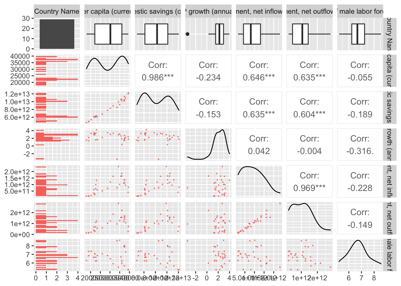
As observed in the scatterplots we find that our covariates have a high correlation with GDP per capita which is promising as we look to begin modeling on this dataset. However, we also notice there is foreign domestic inflow and outflow are very highly correlated. This introduces an issue of collinearity if both are included in a model. To avoid this we remove the variable with a lower correlation with GDP per capita. Additionally, gross domestic savings has a suspiciously high correlation with GDP per capita which makes sense as it is defined as a percentage of GDP. This indicates that our model would be using information is should not have directly available when GDP per capita is our predicted value. Therefore, it should be removed for any subsequent model when predicting GDP per capita.
With these observation we narrow down our covariates (for predicting GDP per capita) to:
- GDP growth (annual %)
- Foreign direct investment inflow or outlflow (TBD)
- Unemployment, male (% of male labor force) (modeled ILO estimate)
This should give us a fair macroeconomic perspective on the economies of both country groups in our dataset.
final_vars = c("Country Name",
               "GDP per capita (current US$)",
               "GDP growth (annual %)",
               "Foreign direct investment, net inflows (BoP, current US$)",
               "Unemployment, male (% of male labor force) (modeled ILO estimate)")
Model Selection
As we determined earlier, we will present a model for each country aggregate to then make comparisions between nations at different stages of economic development. To find the strongest model, we employ backward selection to compare the different choices at hand during model selection.
HIPC Model Selection
#backward selection
wdi_hipc_back <- wdi_econi %>%
  select(final_vars) %>%
  filter(`Country Name`=="Heavily indebted poor countries (HIPC)") %>%
  select(-c(`Country Name`, ))
## Note: Using an external vector in selections is ambiguous.
## ℹ Use `all_of(final_vars)` instead of `final_vars` to silence this message.
## ℹ See <https://tidyselect.r-lib.org/reference/faq-external-vector.html>.
## This message is displayed once per session.models <- regsubsets(`GDP per capita (current US$)`~.,
data = wdi_hipc_back,
nvmax = 3,
method="backward")
summary(models)## Subset selection object
## Call: regsubsets.formula(`GDP per capita (current US$)` ~ ., data = wdi_hipc_back,
## nvmax = 3, method = "backward")
## 3 Variables (and intercept)
## Forced in
## `GDP growth (annual %)` FALSE
## `Foreign direct investment, net inflows (BoP, current US$)` FALSE
## `Unemployment, male (% of male labor force) (modeled ILO estimate)` FALSE
## Forced out
## `GDP growth (annual %)` FALSE
## `Foreign direct investment, net inflows (BoP, current US$)` FALSE
## `Unemployment, male (% of male labor force) (modeled ILO estimate)` FALSE
## 1 subsets of each size up to 3
## Selection Algorithm: backward
## `GDP growth (annual %)`
## 1 ( 1 ) " "
## 2 ( 1 ) " "
## 3 ( 1 ) "*"
## `Foreign direct investment, net inflows (BoP, current US$)`
## 1 ( 1 ) "*"
## 2 ( 1 ) "*"
## 3 ( 1 ) "*"
## `Unemployment, male (% of male labor force) (modeled ILO estimate)`
## 1 ( 1 ) " "
## 2 ( 1 ) "*"
## 3 ( 1 ) "*"summary(models)$cp## [1] 137.744194 6.187641 4.000000summary(models)$adjr2## [1] 0.9512417 0.9909190 0.9919108The model which includes all three covariates has the lowest CP value and highest R^2 so we are comfortable taking this as the model for HIDPC.
OECD Model Selection
#backward selection
wdi_oecd_back <- wdi_econi %>%
  select(final_vars) %>%
  filter(`Country Name`=="OECD members") %>%
  select(-c(`Country Name`, ))

models <- regsubsets(`GDP per capita (current US$)`~.,
                     data = wdi_oecd_back,
                     nvmax = 3,
                     method="backward")
summary(models)
## Subset selection object
## Call: regsubsets.formula(`GDP per capita (current US$)` ~ ., data = wdi_oecd_back,
## nvmax = 3, method = "backward")
## 3 Variables (and intercept)
## Forced in
## `GDP growth (annual %)` FALSE
## `Foreign direct investment, net inflows (BoP, current US$)` FALSE
## `Unemployment, male (% of male labor force) (modeled ILO estimate)` FALSE
## Forced out
## `GDP growth (annual %)` FALSE
## `Foreign direct investment, net inflows (BoP, current US$)` FALSE
## `Unemployment, male (% of male labor force) (modeled ILO estimate)` FALSE
## 1 subsets of each size up to 3
## Selection Algorithm: backward
## `GDP growth (annual %)`
## 1 ( 1 ) " "
## 2 ( 1 ) "*"
## 3 ( 1 ) "*"
## `Foreign direct investment, net inflows (BoP, current US$)`
## 1 ( 1 ) "*"
## 2 ( 1 ) "*"
## 3 ( 1 ) "*"
## `Unemployment, male (% of male labor force) (modeled ILO estimate)`
## 1 ( 1 ) " "
## 2 ( 1 ) " "
## 3 ( 1 ) "*"summary(models)$cp## [1] 3.325707 2.008550 4.000000summary(models)$adjr2## [1] 0.3954681 0.4457350 0.4237615Here we see a difference between OECD countries as the model with Foreign direct investment, net inflows (BoP, current US$) and GDP growth (annual %) does the best according to both CP and R^2 values. A reasonable justification for this is the higher average and higher variance of male unemployment as seen in the trend charts when compared to HIPC group. That may make male unemployment a less valuable covariate for OECD countries.
Final Models
HIPC Model
hipc_final_model <-lm(`GDP per capita (current US$)`~
                 `GDP growth (annual %)` +
                   `Foreign direct investment, net inflows (BoP, current US$)` +
                   `Unemployment, male (% of male labor force) (modeled ILO estimate)`,
              data=wdi_hipc_back)

summary(hipc_final_model)
##
## Call:
## lm(formula = `GDP per capita (current US$)` ~ `GDP growth (annual %)` +
## `Foreign direct investment, net inflows (BoP, current US$)` +
## `Unemployment, male (% of male labor force) (modeled ILO estimate)`,
## data = wdi_hipc_back)
##
## Residuals:
## Min 1Q Median 3Q Max
## -36.66 -16.50 -1.20 15.24 44.34
##
## Coefficients:
## Estimate
## (Intercept) 2.076e+03
## `GDP growth (annual %)` -5.827e+00
## `Foreign direct investment, net inflows (BoP, current US$)` 1.233e-08
## `Unemployment, male (% of male labor force) (modeled ILO estimate)` -3.354e+02
## Std. Error
## (Intercept) 1.541e+02
## `GDP growth (annual %)` 2.848e+00
## `Foreign direct investment, net inflows (BoP, current US$)` 9.749e-10
## `Unemployment, male (% of male labor force) (modeled ILO estimate)` 2.922e+01
## t value
## (Intercept) 13.468
## `GDP growth (annual %)` -2.046
## `Foreign direct investment, net inflows (BoP, current US$)` 12.652
## `Unemployment, male (% of male labor force) (modeled ILO estimate)` -11.477
## Pr(>|t|)
## (Intercept) 5.83e-13
## `GDP growth (annual %)` 0.0514
## `Foreign direct investment, net inflows (BoP, current US$)` 2.29e-12
## `Unemployment, male (% of male labor force) (modeled ILO estimate)` 1.85e-11
##
## (Intercept) ***
## `GDP growth (annual %)` .
## `Foreign direct investment, net inflows (BoP, current US$)` ***
## `Unemployment, male (% of male labor force) (modeled ILO estimate)` ***
## ---
## Signif. codes: 0 '***' 0.001 '**' 0.01 '*' 0.05 '.' 0.1 ' ' 1
##
## Residual standard error: 24.07 on 25 degrees of freedom
## Multiple R-squared: 0.9928, Adjusted R-squared: 0.9919
## F-statistic: 1145 on 3 and 25 DF, p-value: < 2.2e-16OECD Model
oecd_final_model <- lm(`GDP per capita (current US$)`~
                 `GDP growth (annual %)` +
                   `Foreign direct investment, net inflows (BoP, current US$)`,
              data=wdi_oecd_back)

summary(oecd_final_model)
##
## Call:
## lm(formula = `GDP per capita (current US$)` ~ `GDP growth (annual %)` +
## `Foreign direct investment, net inflows (BoP, current US$)`,
## data = wdi_oecd_back)
##
## Residuals:
## Min 1Q Median 3Q Max
## -7072 -4033 -1369 3948 14297
##
## Coefficients:
## Estimate
## (Intercept) 2.459e+04
## `GDP growth (annual %)` -1.461e+03
## `Foreign direct investment, net inflows (BoP, current US$)` 8.606e-09
## Std. Error t value
## (Intercept) 2.510e+03 9.797
## `GDP growth (annual %)` 7.866e+02 -1.857
## `Foreign direct investment, net inflows (BoP, current US$)` 1.846e-09 4.663
## Pr(>|t|)
## (Intercept) 3.25e-10 ***
## `GDP growth (annual %)` 0.0747 .
## `Foreign direct investment, net inflows (BoP, current US$)` 8.18e-05 ***
## ---
## Signif. codes: 0 '***' 0.001 '**' 0.01 '*' 0.05 '.' 0.1 ' ' 1
##
## Residual standard error: 5578 on 26 degrees of freedom
## Multiple R-squared: 0.4853, Adjusted R-squared: 0.4457
## F-statistic: 12.26 on 2 and 26 DF, p-value: 0.0001778This OECD model has a moderate-low fit to the data as indicated by the R squared value. Looking back to the trends we see that GDP per capita levels off after a period of fast growth. As these countries are more developed the GDP appears to be approaching saturation so a logarithmic model may be more appropriate.
OECD Model on log(GDP per Capita)
oecd_final_model <- lm(log(`GDP per capita (current US$)`)~
                 `GDP growth (annual %)` + `Foreign direct investment, net inflows (BoP, current US$)`,
              data=wdi_oecd_back)

summary(oecd_final_model)
##
## Call:
## lm(formula = log(`GDP per capita (current US$)`) ~ `GDP growth (annual %)` +
## `Foreign direct investment, net inflows (BoP, current US$)`,
## data = wdi_oecd_back)
##
## Residuals:
## Min 1Q Median 3Q Max
## -0.25725 -0.13923 -0.04102 0.12982 0.48549
##
## Coefficients:
## Estimate
## (Intercept) 1.007e+01
## `GDP growth (annual %)` -4.962e-02
## `Foreign direct investment, net inflows (BoP, current US$)` 3.190e-13
## Std. Error t value
## (Intercept) 8.715e-02 115.517
## `GDP growth (annual %)` 2.732e-02 -1.816
## `Foreign direct investment, net inflows (BoP, current US$)` 6.409e-14 4.977
## Pr(>|t|)
## (Intercept) < 2e-16 ***
## `GDP growth (annual %)` 0.0808 .
## `Foreign direct investment, net inflows (BoP, current US$)` 3.57e-05 ***
## ---
## Signif. codes: 0 '***' 0.001 '**' 0.01 '*' 0.05 '.' 0.1 ' ' 1
##
## Residual standard error: 0.1937 on 26 degrees of freedom
## Multiple R-squared: 0.5128, Adjusted R-squared: 0.4753
## F-statistic: 13.68 on 2 and 26 DF, p-value: 8.719e-05The results from the logarithmic model above does show improvement - both in the r squared value and the global F-test p-value. This indicates that predicting on the log GDP per capita is probably a better approach.
Final Thoughts
The data exploration and subsequent modeling above reveal some differences between OECD and HIPC countries. As we deal with macroeconomic coviarates we can ony discuss these differences at the macro level. Most notably, OECD models appear to reach a more stable economic level which makes unemployment predictors less useful in modeling. Furthermore, we also further justification for these assessment as we see improvment when modeling the log per capita which enforces this assumption about the more mature OECD countries. As for HIPC countries we see a very very strong correlation with foreign direct investment which seems to indicate that this investment pays off in the form of GDP per capita increase (positive coefficient is present). Overall, this analysis illustrates some key difference between our two country groups and would be a good start to someone learning about macroeconomic policy and investment.
FDI Analysis
All the variables we use for this analysis, including:
GDP per capita (current US$)
Gross domestic savings (current US$)
GDP growth (annual %)
Foreign direct investment, net inflows (BoP, current US$)
Foreign direct investment, net outflows (BoP, current US$)
Unemployment, male (% of male labor force) (modeled ILO estimate)
Number of Infant Deaths: Mortality Rate (under 5 per 1,000 live births)
Rural population (% of total population)
Primary school enrollment (% gross)
Unemployment, male (% of male labor force)
We start by visualizing how the different FDI (inflow/outflow) of HIPC and OECD countries changes according to the time from 1990 to 2020.
econi$count = as.numeric(econi$count)
summ <- function(x){
  sum(x,na.rm = TRUE)
}
Trend_time <- econi%>%mutate(years = as.numeric(year))%>%
  filter(`Indicator Name` == "Foreign direct investment, net outflows (BoP, current US$)"
         |`Indicator Name` == "Foreign direct investment, net inflows (BoP, current US$)")
Trend_time%>%ggplot(aes(x = years, y= count)) + geom_point(aes(color = `Indicator Name`),size = 1, alpha = 0.7) +
  facet_wrap(`Country Name`~`Indicator Name`, scales = "free") +
  geom_smooth(method = lm, se = T, fullrange =TRUE, color = "Red")
## `geom_smooth()` using formula 'y ~ x'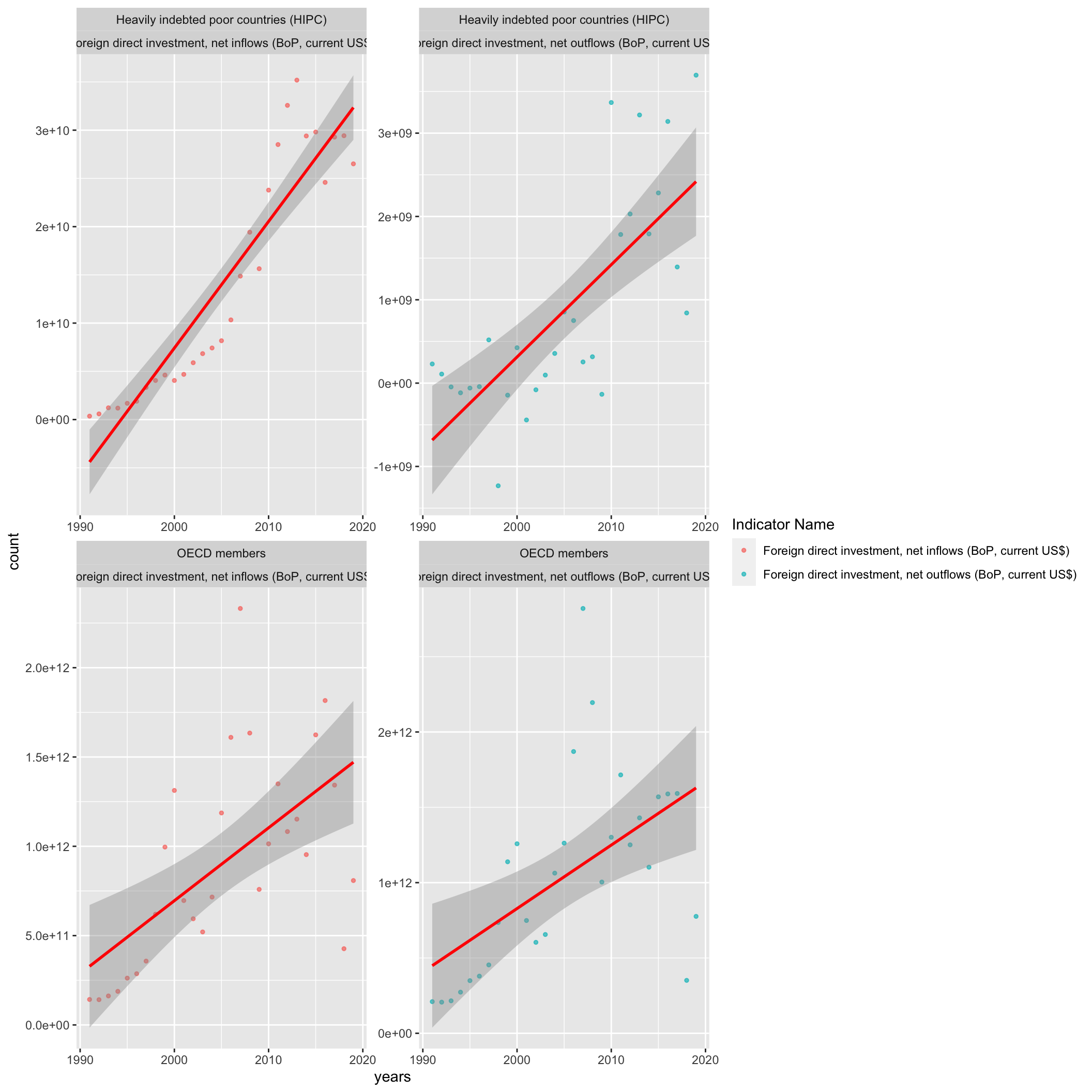 As the plots show above, FDI values have an increasing trend over time. What is
also interesting to see is the flatter trend line for OECD countries. We deduce
this to be a result of lower FDI levels in developed countries, as high levels of
investment is normally conducted in low-income places ripe for growth.
In order to have more detailed view of how other variable impact FDI, we need to
combine FDI net outflows and FDI net inflows to a single response variable “FDI”.
By definition, FDI net inflows are the value of inward direct investment made by
non-resident investors in the reporting economy.
FDI net outflows are the value of outward direct investment made by the residents
of the reporting economy to external economies.
We calculate the FDI net flows as FDI net inflows minus FDI net outflows.
As the plots show above, FDI values have an increasing trend over time. What is
also interesting to see is the flatter trend line for OECD countries. We deduce
this to be a result of lower FDI levels in developed countries, as high levels of
investment is normally conducted in low-income places ripe for growth.
In order to have more detailed view of how other variable impact FDI, we need to
combine FDI net outflows and FDI net inflows to a single response variable “FDI”.
By definition, FDI net inflows are the value of inward direct investment made by
non-resident investors in the reporting economy.
FDI net outflows are the value of outward direct investment made by the residents
of the reporting economy to external economies.
We calculate the FDI net flows as FDI net inflows minus FDI net outflows.
In order to have the model which can predict the FDI well, we visualize those correlations that corresponding to FDI separately in HPC and OECD countries,which provide the insights into which variables are adequate for predicting FDI:
#calculate and visulize the correlation for HPC FDI vs
#first step is to calculate the net FDI value
Trend_HPC<- econi%>%pivot_wider(names_from = `Indicator Name`, values_from = `count`)%>%
  mutate(FDI = `Foreign direct investment, net inflows (BoP, current US$)`-`Foreign direct investment, net outflows (BoP, current US$)`)%>%
  select(-`Foreign direct investment, net inflows (BoP, current US$)`,-`Foreign direct investment, net outflows (BoP, current US$)`)%>%
  filter(`Country Name` == "Heavily indebted poor countries (HIPC)")%>%
  pivot_longer(cols = !all_of(c("year", "Country Name", "FDI")), names_to = "Indicator Name", values_to = "Indicator Value")
#calculate the correlation for each set
Corr_df_HPC <- Trend_HPC %>% group_by(`Indicator Name`)%>%
  nest() %>%
  mutate(Mod = map(data, ~lm(`FDI` ~ `Indicator Value`, data = .x))) %>%
  mutate(Cor_r2 = map_dbl(Mod, ~round(summary(.x)$r.squared, 3)))
#visulize
Trend_HPC%>%ggplot(aes(x = `Indicator Value`, y = FDI))+ geom_point() +
  geom_smooth(method = lm, se = T, fullrange =TRUE, color = "blue") +
  geom_label(data = Corr_df_HPC,
             aes(x = Inf, y = Inf,
                 label = paste("Corr R2 = ", Cor_r2, sep = " ")),
             hjust = 1, vjust = 1) +
  facet_wrap(`Indicator Name`~ ., scales = "free")
## `geom_smooth()` using formula 'y ~ x'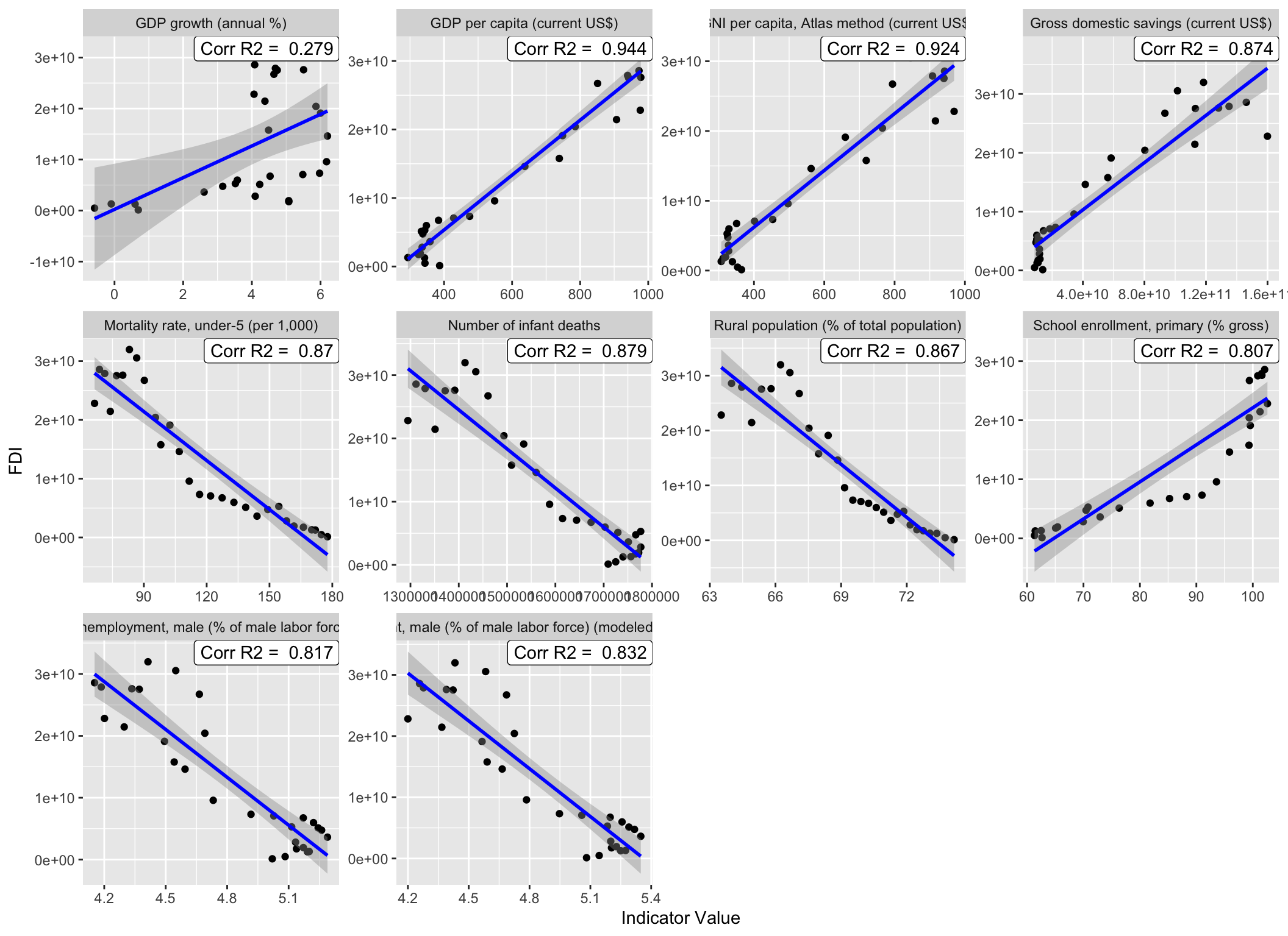
From the graph above (except the correlations of FDI net inflows and out flows), we know that the FDI is highly correlated to the annual GDP growth in HPC, which indicate that “GDP per capita (current US$)” might be one of the predictors in our final model of predicting FDI.
We continue to conduct the same method of finding out the correlations for OECD countries:
#calculate and visulize the correlation for HPC FDI vs
#first step is to calculate the net FDI value
Trend_OECD<- econi%>%pivot_wider(names_from = `Indicator Name`, values_from = `count`)%>%
  mutate(FDI = `Foreign direct investment, net inflows (BoP, current US$)` -`Foreign direct investment, net outflows (BoP, current US$)`)%>%
  select(-`Foreign direct investment, net inflows (BoP, current US$)`,-`Foreign direct investment, net outflows (BoP, current US$)`)%>%
  filter(`Country Name` == "OECD members")%>%
  pivot_longer(cols = !all_of(c("year", "Country Name", "FDI")), names_to = "Indicator Name", values_to = "Indicator Value")
#calculate the correlation for each set


Corr_df_HPC <- Trend_OECD %>% group_by(`Indicator Name`)%>%
  nest() %>%
  mutate(Mod = map(data, ~lm(`FDI` ~ `Indicator Value`, data = .x))) %>%
  mutate(Cor_r2 = map_dbl(Mod, ~round(summary(.x)$r.squared, 3)))
#visulize
Trend_OECD%>%ggplot(aes(x = `Indicator Value`, y = FDI))+ geom_point() +
  geom_smooth(method = lm, se = T, fullrange =TRUE, color = "red") +
  geom_label(data = Corr_df_HPC,
             aes(x = Inf, y = Inf,
                 label = paste("Corr R2 = ", Cor_r2, sep = " ")),
             hjust = 1, vjust = 1) +
  facet_wrap(`Indicator Name`~ ., scales = "free")
## `geom_smooth()` using formula 'y ~ x'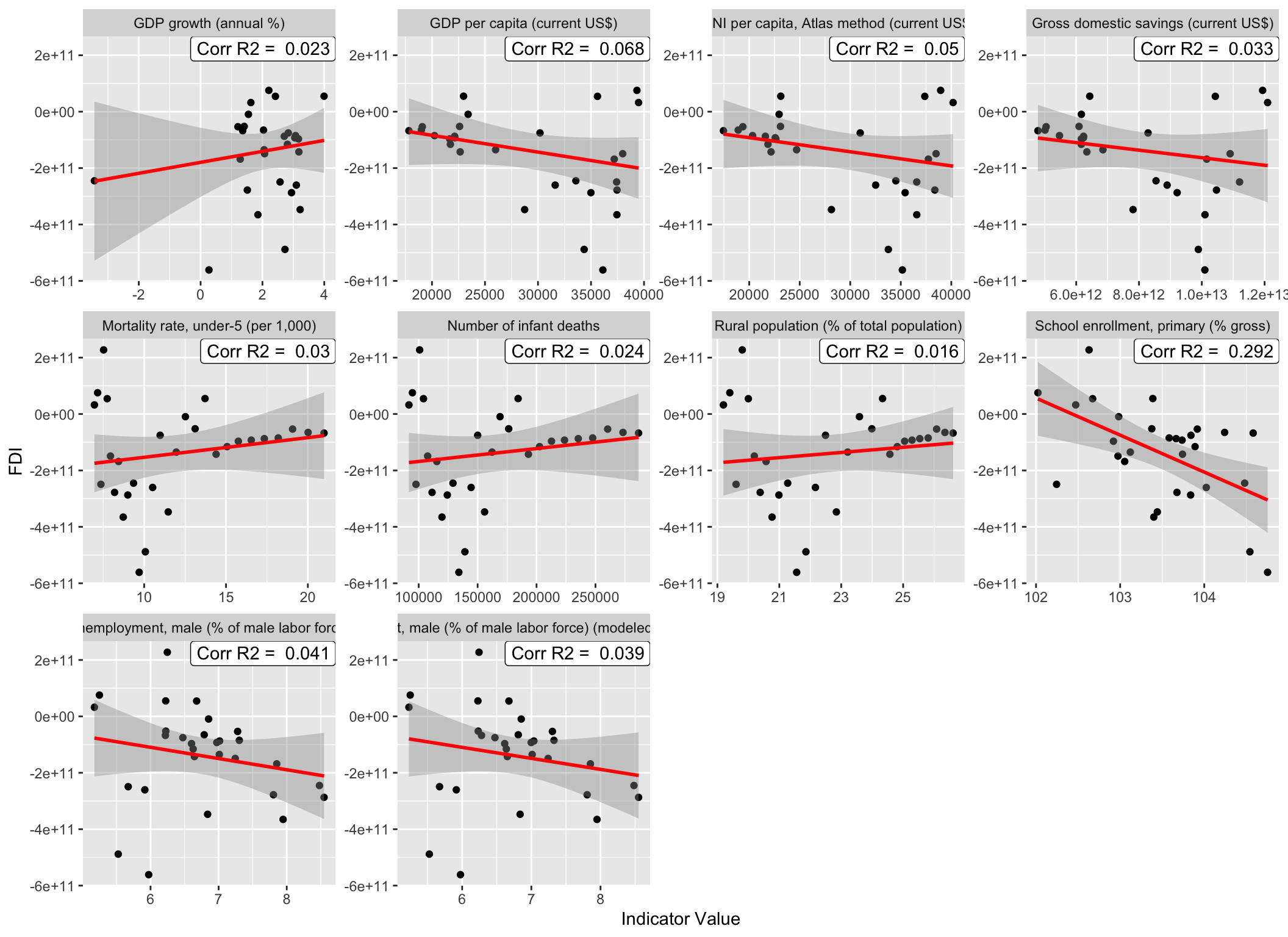 Compared with those correlations of HPC countries, there are
less significant correlations found in OECD countries,
which lead our suspicion that using the matrices above to
predict FDI of OECD will have larger errors compare to predicting FDI of HPC.
Compared with those correlations of HPC countries, there are
less significant correlations found in OECD countries,
which lead our suspicion that using the matrices above to
predict FDI of OECD will have larger errors compare to predicting FDI of HPC.
Now, in this part, we select the model for predicting FDI in HPC and OECD by using different schemes, including BIC, CP, ADJR2, and our cross-validation method.
HIPC Model on FDI prediction
#data manipulation for modeling
#HPC
HPC_DF<- econi%>%pivot_wider(names_from = `Indicator Name`, values_from = `count`)%>%
  mutate(year = as.numeric(year),FDI = `Foreign direct investment, net inflows (BoP, current US$)` -`Foreign direct investment, net outflows (BoP, current US$)`)%>%
  filter(`Country Name` == "Heavily indebted poor countries (HIPC)")%>%
  select(-`Country Name`,-`Foreign direct investment, net inflows (BoP, current US$)`,-`Foreign direct investment, net outflows (BoP, current US$)`)    #exclude the covariate of country name
#OECD
OECD_DF<- econi%>%pivot_wider(names_from = `Indicator Name`, values_from = `count`)%>%
  mutate(year = as.numeric(year),FDI = `Foreign direct investment, net inflows (BoP, current US$)` -`Foreign direct investment, net outflows (BoP, current US$)`)%>%
  filter(`Country Name` == "OECD members")%>%
  select(-`Country Name`,-`Foreign direct investment, net inflows (BoP, current US$)`,-`Foreign direct investment, net outflows (BoP, current US$)`)    #exclude the covariate of country name

#best model subsets using the whole Data set
Models_HPC <- regsubsets(`FDI`~., data = HPC_DF, method = "exhaustive", nvmax = 11) #11 variables Using exhaustive method
#coef(Models_HPC,which.min(summary(Models_HPC)$cp))


bestbic <- which.min(summary(Models_HPC)$bic)
bestcp <- which.min(summary(Models_HPC)$cp)
bestadjr2 <- which.max(summary(Models_HPC)$adjr2)
plot(summary(Models_HPC)$bic,xlab='number of predictors',ylab='HPC_FDI_BIC',type='l')
points(bestbic,summary(Models_HPC)$bic[bestbic],pch=19,col='red')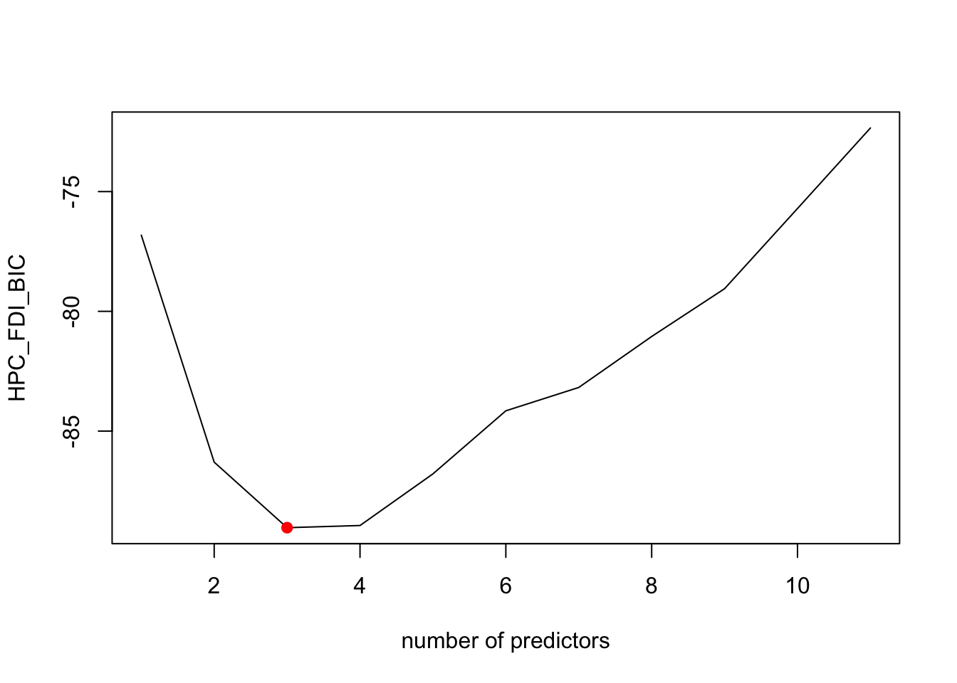
plot(summary(Models_HPC)$cp,xlab='number of predictors',ylab='HPC_FDI_CP',type='l')
points(bestcp,summary(Models_HPC)$cp[bestcp],pch=19,col='red')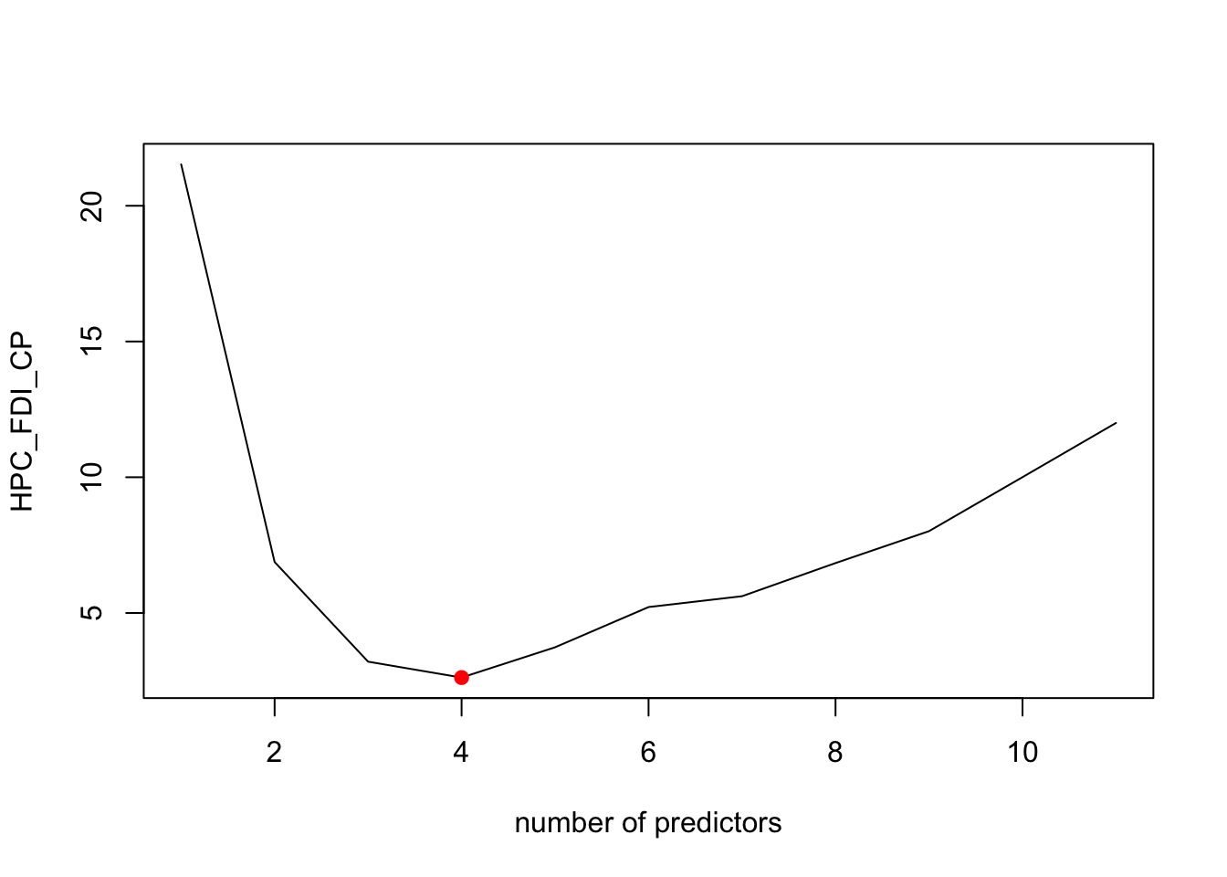
plot(summary(Models_HPC)$adjr2,xlab='number of predictors',ylab='HPC_FDI_ADJR2',type='l')
points(bestadjr2,summary(Models_HPC)$adjr2[bestadjr2],pch=19,col='red')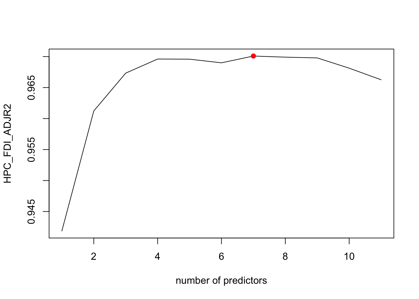
#coef(Models_HPC,which.min(summary(Models_HPC)$bic))
#coef(Models_HPC,which.min(summary(Models_HPC)$cp))
#coef(Models_HPC,which.max(summary(Models_HPC)$adjr2))
#coef(Models_HPC,4)
####
predict.regsubsets <- function(object, newdata, id ,...) {
  form <- as.formula(object$call[[2]])
  mat <- model.matrix(form, newdata)
  coefi <- coef(object, id = id)
  xvars <- names(coefi)
  mat[, xvars] %*% coefi
}
####
#perform cross-validatation to select number perdictors for the model
k <- 14   #fold 14 times
set.seed(1)
folds <- sample(1:k, nrow(HPC_DF), replace = TRUE)
cv_errors <- matrix(NA, k, 11, dimnames = list(NULL, paste(1:11))) #store errors
for(j in 1:k) {
  best_subset <- regsubsets(FDI ~ ., HPC_DF[folds != j, ], nvmax = 11) #remainder in training set

  #cross-validation
  for( i in 1:11) {
    pred_x <- predict.regsubsets(best_subset, HPC_DF[folds == j, ], id = i)
    cv_errors[j, i] <- mean((HPC_DF$FDI[folds == j] - pred_x)^2)
    }
}
# plot the cv mse
mean_cv_errors <- colMeans(cv_errors, na.rm = TRUE)
plot(mean_cv_errors, type = "l")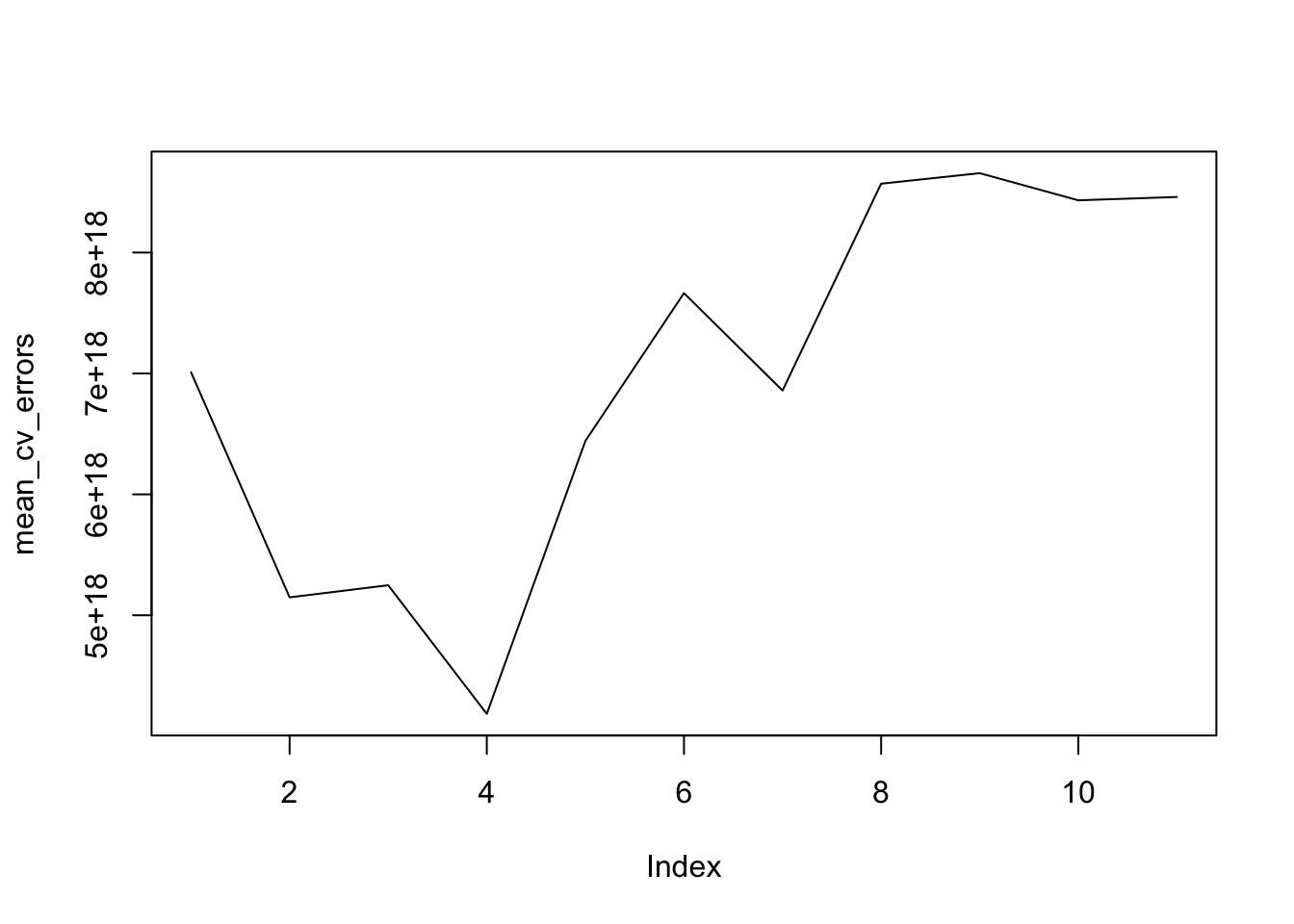
best_model_error_HPC <- mean_cv_errors[4]According to the plot above, the best model for CP criterion has 4 predictors, as well as our cross-validation approach, On the other hand, the adjr2 suggests 7 predictors, and Bic indicate 3.
However, these four models all have the predictors of “GDP per capita (current US$)”, “Unemployment, male (% of male labor force) (modeled ILO estimate)”, which suggest that those two coefficients has relative stronger linear relationships when predicting the FDI in HPC countries.
Thus, the best model for predicting FDI of HPC is -6.939741^{10}, 1.0099118^{8}, 1.8405505^{10}, -4.3266692^{7}, -6.1084578^{8} and the best MSE error is 4.1844762^{18}
We do the same thing for predicting FDI in OECD countries.
OECD Model on FDI prediction
#best model subsets using the whole Data set
Models_OECD <- regsubsets(`FDI`~., data = OECD_DF, method = "exhaustive", nvmax = 11) #11 variables Using exhaustive method
bestbic <- which.min(summary(Models_OECD)$bic)
bestcp <- which.min(summary(Models_OECD)$cp)
bestadjr2 <- which.max(summary(Models_OECD)$adjr2)
plot(summary(Models_OECD)$bic,xlab='number of predictors',ylab='HPC_FDI_BIC',type='l')
points(bestbic,summary(Models_OECD)$bic[bestbic],pch=19,col='red')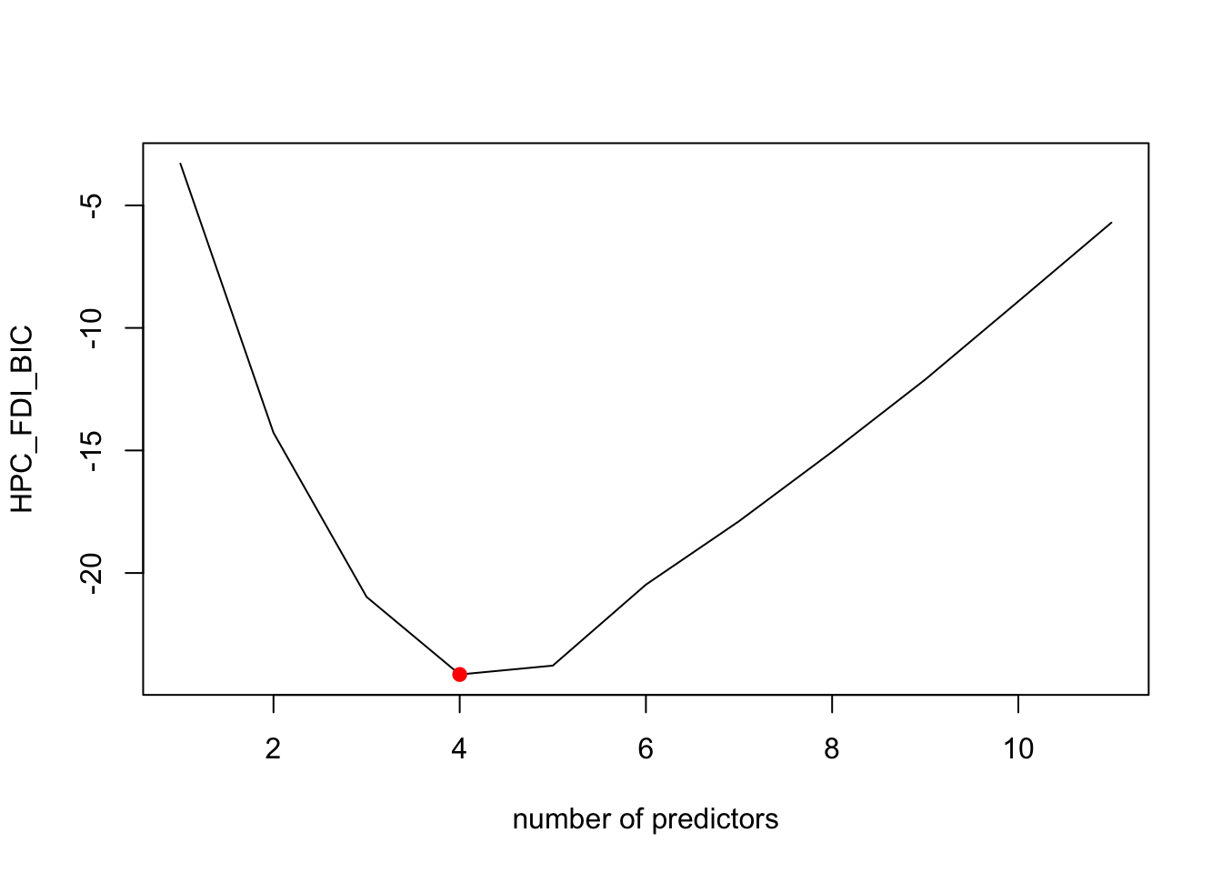
plot(summary(Models_OECD)$cp,xlab='number of predictors',ylab='HPC_FDI_CP',type='l')
points(bestcp,summary(Models_OECD)$cp[bestcp],pch=19,col='red')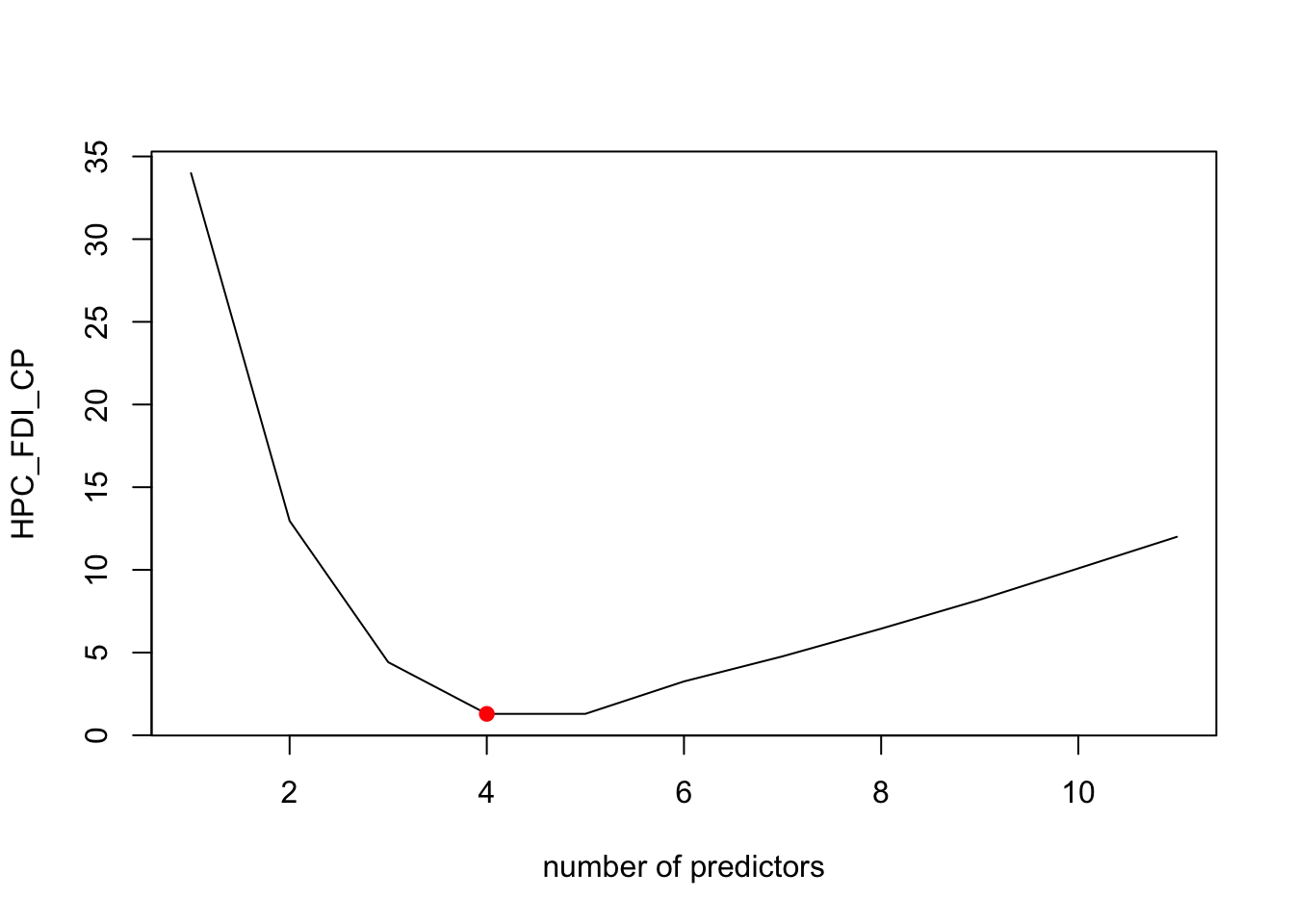
plot(summary(Models_OECD)$adjr2,xlab='number of predictors',ylab='HPC_FDI_ADJR2',type='l')
points(bestadjr2,summary(Models_OECD)$adjr2[bestadjr2],pch=19,col='red')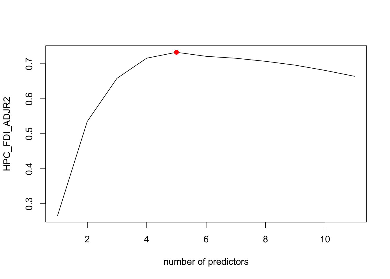
#perform cross-validatation to select number perdictors for the model
k <- 14   #fold 14 times
set.seed(1)
folds <- sample(1:k, nrow(OECD_DF), replace = TRUE)
cv_errors <- matrix(NA, k, 11, dimnames = list(NULL, paste(1:11))) #store errors
for(j in 1:k) {
  best_subset <- regsubsets(FDI ~ ., OECD_DF[folds != j, ], nvmax = 11) #remainder in training set

  #cross-validation
  for( i in 1:11) {
    pred_x <- predict.regsubsets(best_subset, OECD_DF[folds == j, ], id = i)
    cv_errors[j, i] <- mean((OECD_DF$FDI[folds == j] - pred_x)^2)
    }
}
# plot the cv mse
mean_cv_errors <- colMeans(cv_errors, na.rm = TRUE)
plot(mean_cv_errors, type = "l")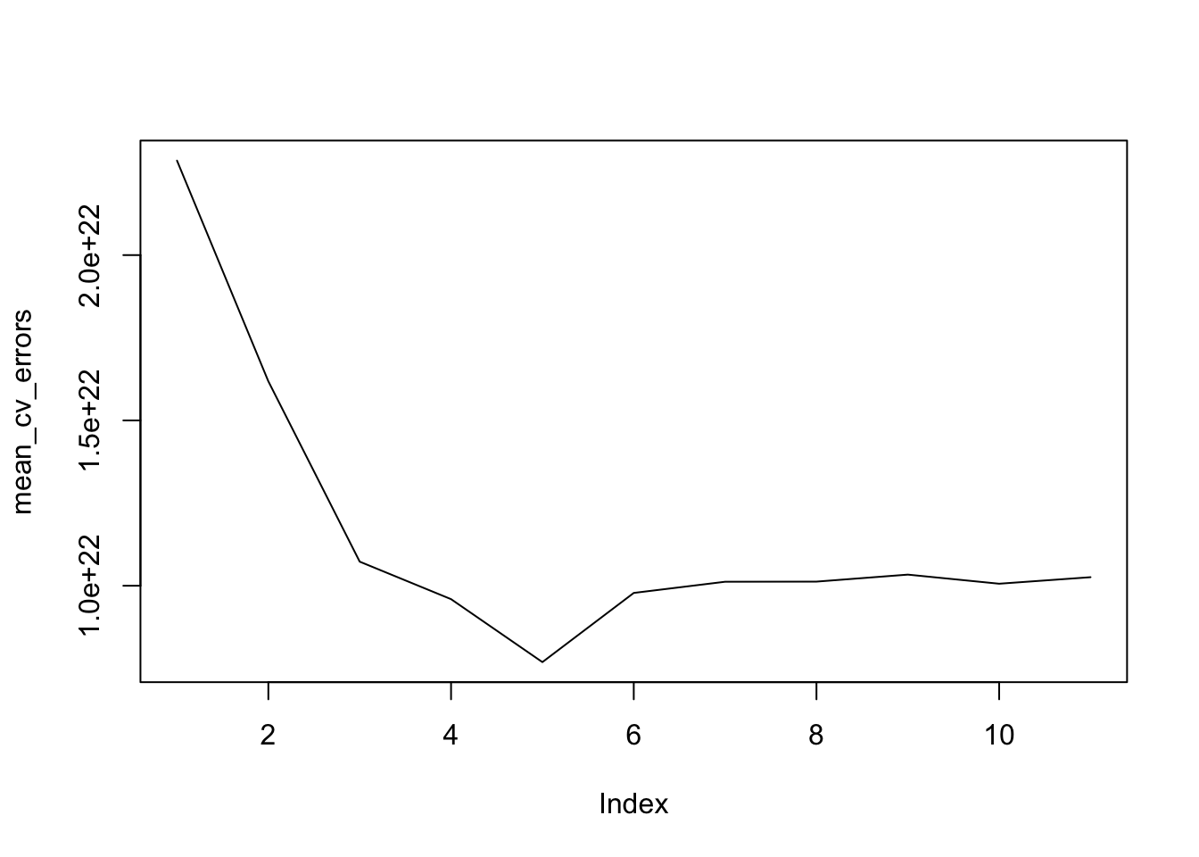
best_model_error_OECD <- mean_cv_errors[5]The best MSE error is 7.6901504^{21}, with the 5 predictors model that -1.0706761^{14}, 5.7382116^{10}, -1.1035892^{8}, 6.5940821^{7}, 3.79929^{6}, -7.1995139^{10}. Comparing it with 4.1844762^{18}, the error for predicting FDI in OECD country is significant larger, which is due to that less correlation of FDI to the other matrices found in the OECD countries.
Final Thoughts
In this section, we are using the microeconomic and macroeconomic factors as predictor variable to conduct the FDI analysis in HPC and OECD countries.
We start by plotting the trend of FDI versus time, which both types of country generally has increasing FDI trend over the time period, and provide us some insights of the FDI, but cannot give us the specific useful information regrading the FDI prediction.
Then, we plot all the other FDI correlations of HPC and OECD, and find out that the GDP per capita has the strongest correlation to FDI, and we make the assumption that the GDP per capita should be including in our final prediction model. Also, it is worth noting that, comparing to those of HPC, less significant correlations of FDI are found in OECD countries, which lead our hypothesis that our final model will generate larger error when predict FDI in OECD.
Next, we use the regsubset method to find the best subset models for our FDI prediction, and we determine that the 4 predictors in HPC Model and 5 predictors in OECD Model are the best overall. Also, the error in OECD Model is larger than those in HPC Model, which confirm our previous hypothesis, and imply that OECD countries’ FDI generally has less dependency on the matrices we use in this analysis.
Although our models could not predict FDI in HPC and OECD precisely, the models provide us the insights that how the given variables relate to the FDI in HPC and OECD.
Microeconomic Variable Analysis
In this part of the analysis, we focus on microeconomic metrics. To conduct a holistic economic analysis, we joined an external dataset which focused on standard of living and quality of life measure for individuals. Following the prior analyses, we differentiate between different environments by looking at a set of developing (HIPC) and developed (OECD) countries.
To get started, we shortened to dataset to the microeconomic variables of interest. These variables are:
- Number of Infant Deaths: Mortality Rate (under 5 per 1,000 live births)
- Rural population (% of total population)
- Primary school enrollment (% gross)
- Unemployment, male (% of male labor force)
Notes on this dataset:
School Enrollment has values of over 100% as it is calculated for student of all ages. Since this variables measures primary school enrollment, the a lot of the data collected is from individuals above the primary school age group.
Unemployment data for females was scarce and difficult to use for analysis. Therefore, we decided to use solely male data.
#filtering out the macro covariates
micov<-c("Number of infant deaths",
              "Rural population (% of total population)",
              "School enrollment, primary (% gross)",
              "Unemployment, male (% of male labor force)",
         "GDP per capita (current US$)",
         "year",
         "Country Name")
micro_econi<-select(econi_wide,micov)
## Note: Using an external vector in selections is ambiguous.
## ℹ Use `all_of(micov)` instead of `micov` to silence this message.
## ℹ See <https://tidyselect.r-lib.org/reference/faq-external-vector.html>.
## This message is displayed once per session.Given that we are now working on a microeconomic level, we must adjust our analysis. Primarily, GDP per capita can no longer be our response variable. Comparing microeconomic variables to macroeconomic outcome is a difficult task and requires a large level of inference. Keeping this in mind, we have decided to use Unemployment as our target variable. There are many reasons for this:
- Unemployment is a variable whose effects can be linked (through complex economic models) to GDP and other developmental measures. This makes any conclusions we make in this part adequate for extrapolation to a macro setting.
- Unemployment encompasses the general education levels of a population and also provides an insight into income levels (and therefore standard of living measures). This makes it perfect for our analysis.
To get an idea of how these values are distributed over time, we take a look at the following scatter plots:
#trend over time

par(mfrow=c(1,4))
micro_econi %>% group_by(`Country Name`) %>%
  ggplot(aes(x=year,
             y=`Unemployment, male (% of male labor force)`,
             col=`Country Name`)) +
geom_point() 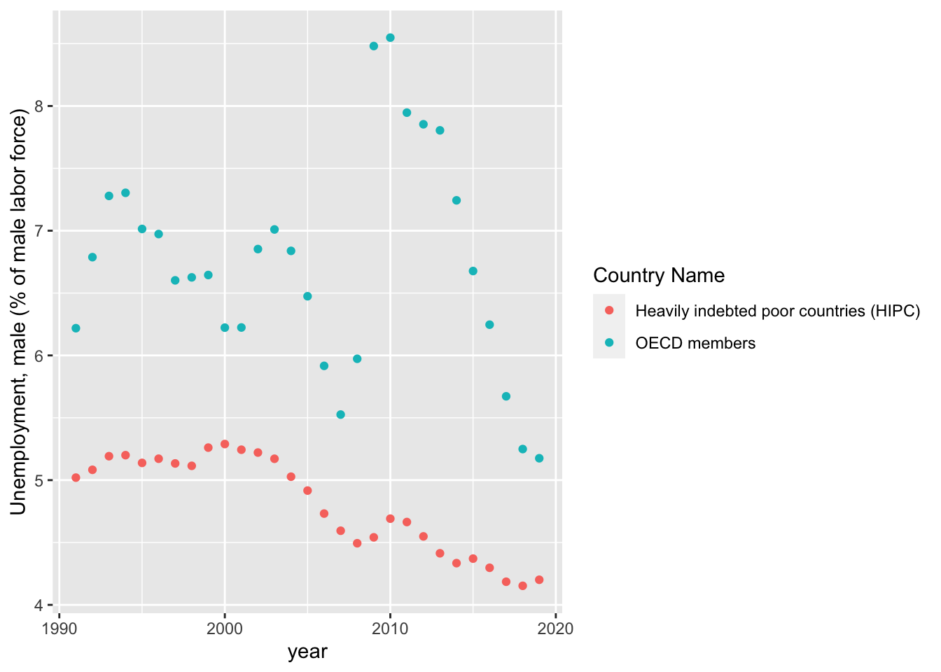
micro_econi %>% group_by(`Country Name`) %>%
  ggplot(aes(x=year,
             y=`School enrollment, primary (% gross)`,
             col=`Country Name`)) +
geom_point() 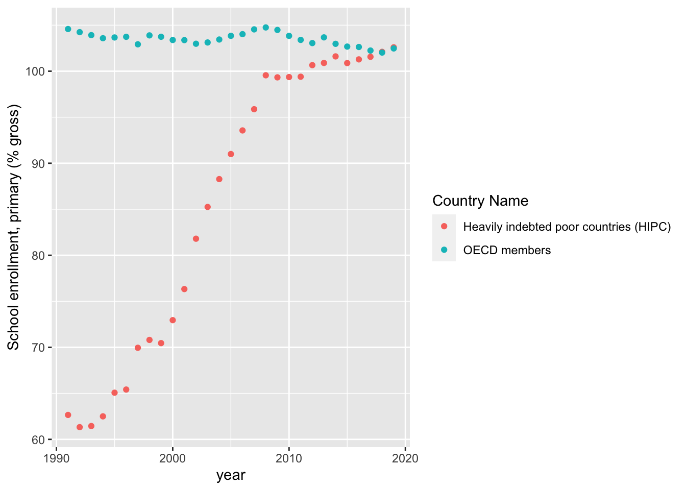
micro_econi %>% group_by(`Country Name`) %>%
  ggplot(aes(x=year,
             y=`Rural population (% of total population)`,
             col=`Country Name`)) +
geom_point() 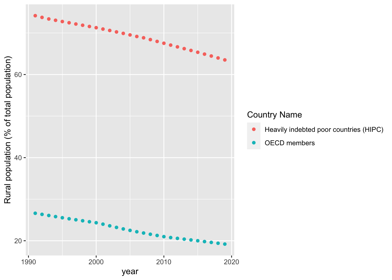
micro_econi %>% group_by(`Country Name`) %>%
  ggplot(aes(x=year,
             y=`Number of infant deaths`,
             col=`Country Name`)) +
geom_point() 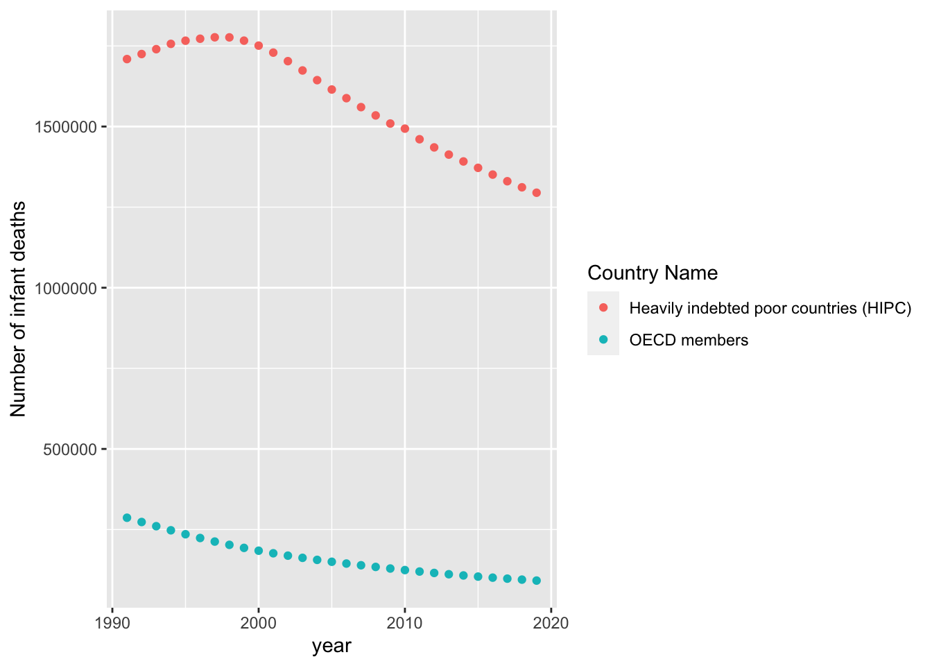
Let’s take a look at which variables are most closely correlated to Unemployment. We first look at the correlations between all covariates:
#lets look at which variables are most closely correlated to GDP per capita (the main focus of this study)
#together
meic_mod_all<-micro_econi %>% select(-year)
scatter_all<-ggpairs(meic_mod_all,
        progress = F,
        lower = list(continuous = wrap("points", alpha = 0.8,    size=0.2),
                     mapping=ggplot2::aes(colour=micro_econi$`Country Name`))) +
  theme(legend.position = "bottom")
While the scatterplot matrix is slightly difficult to read, the main goal of this figure is to look at the distribution of values for each country. Taking an enhanced look at the boxplots:
#distribution of values
par(mfrow=c(1,5))
getPlot(scatter_all, 1, 6) + guides(fill=FALSE)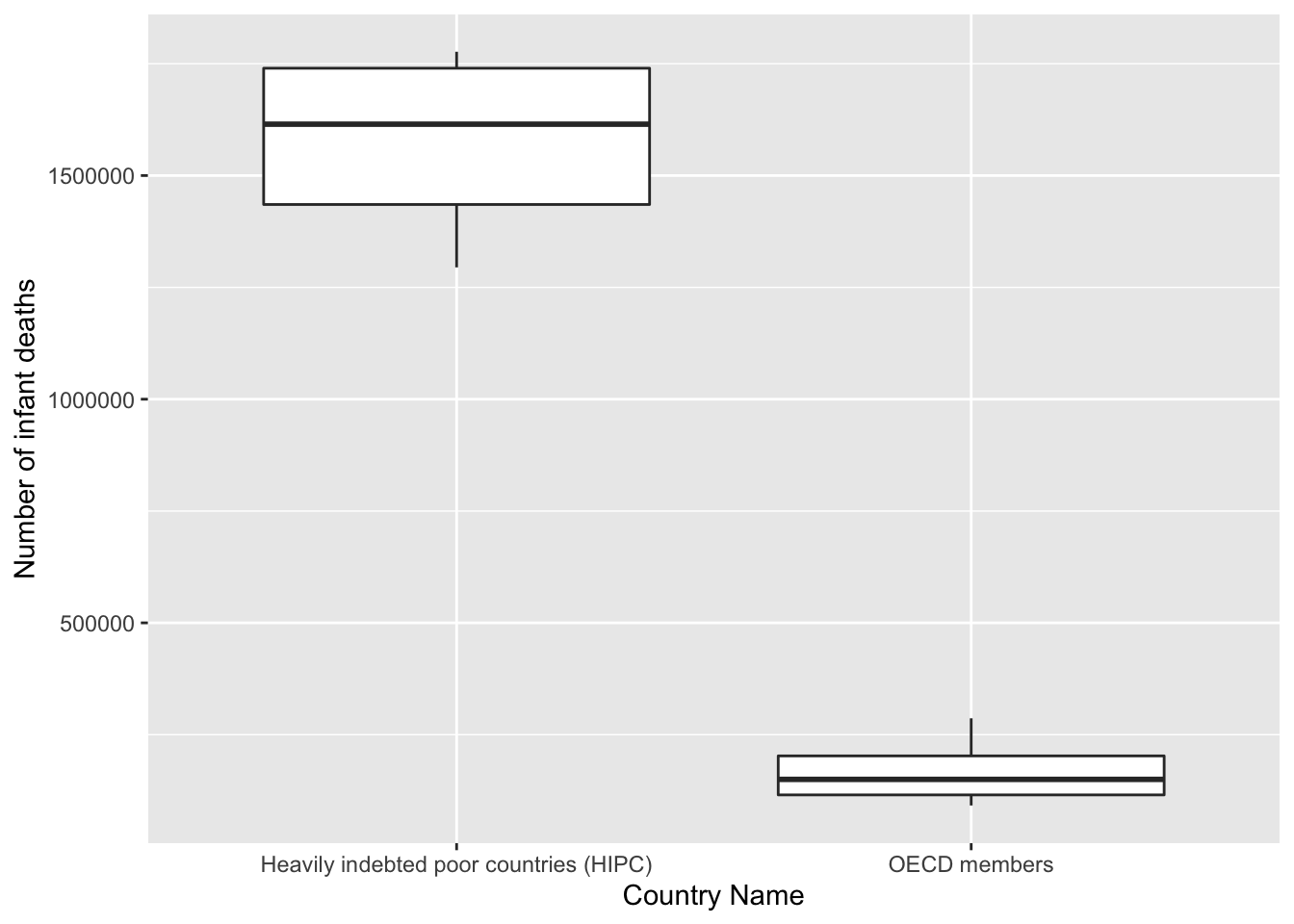
getPlot(scatter_all, 2, 6) + guides(fill=FALSE)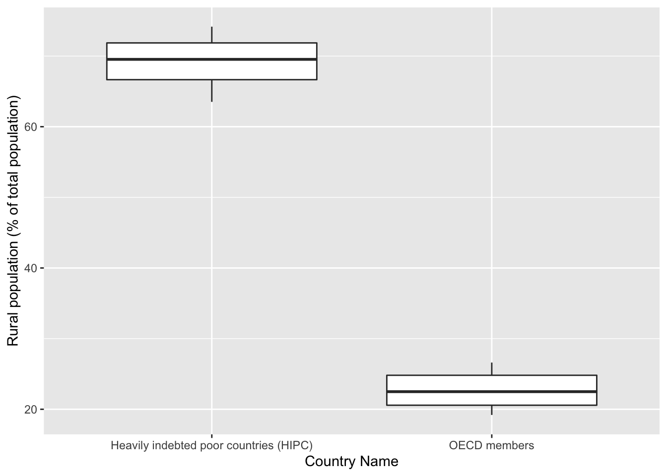
getPlot(scatter_all, 3, 6) + guides(fill=FALSE)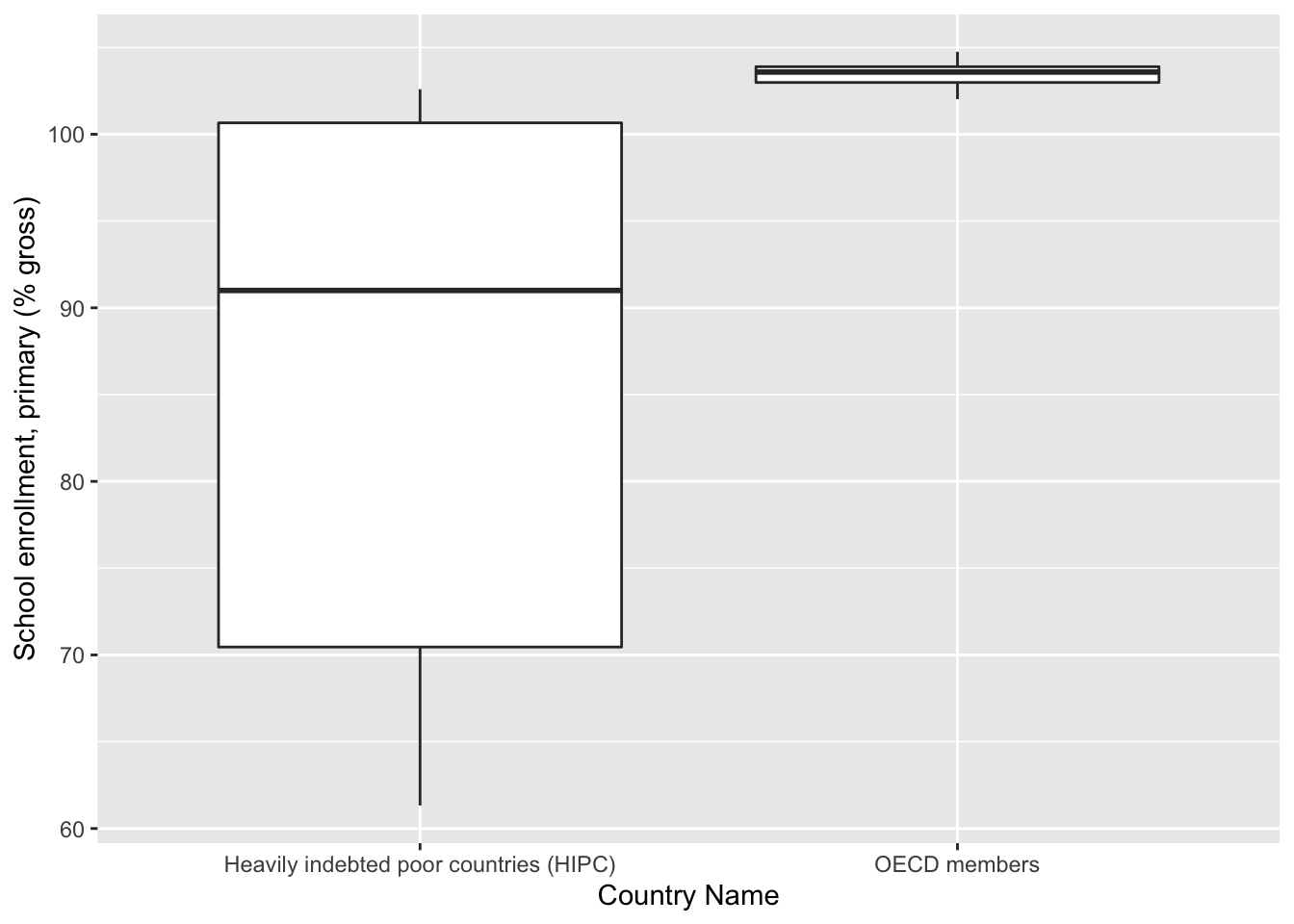
getPlot(scatter_all, 4, 6) + guides(fill=FALSE)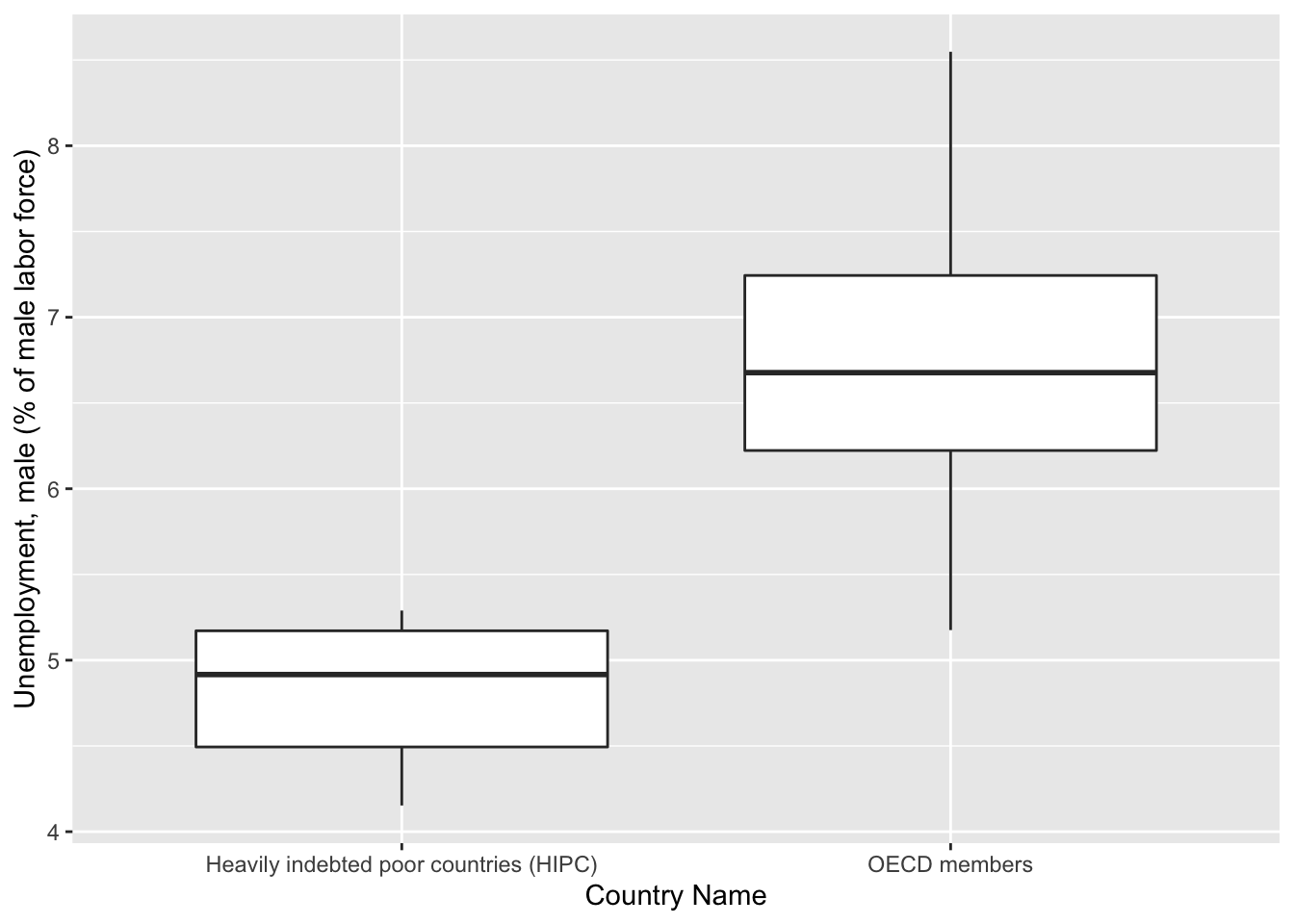
getPlot(scatter_all, 5, 6) + guides(fill=FALSE)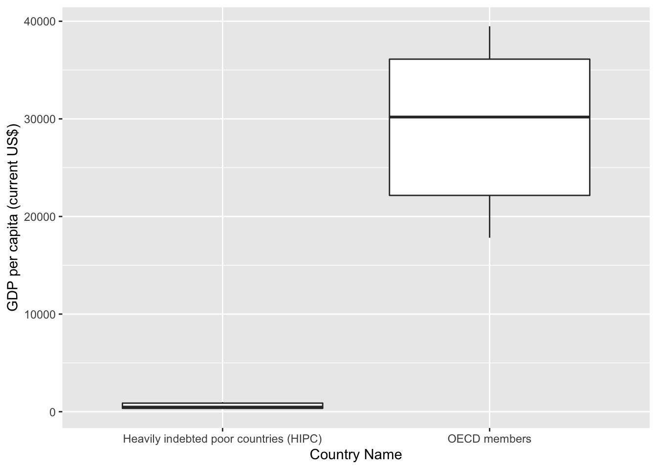 From these boxplots, we can see that there is a large disparity for each metric
between HIPC and OECD countries. This gives us an indication that we have to
conduct separate analyses for both sets of countries.
From these boxplots, we can see that there is a large disparity for each metric
between HIPC and OECD countries. This gives us an indication that we have to
conduct separate analyses for both sets of countries.
We start by looking at the scatterplot matrix, this time for each set of countries starting with HIPC:
#HIPC
miec_mod_hipc<-micro_econi %>%
  filter(`Country Name` == "Heavily indebted poor countries (HIPC)")
miec_mod_hipc<-
  select(miec_mod_hipc,-c(year, `Country Name`,`GDP per capita (current US$)`))

ggpairs(miec_mod_hipc,
        progress = F,
        lower = list(continuous = wrap("points", alpha = 0.8, size=0.2,colour="red")))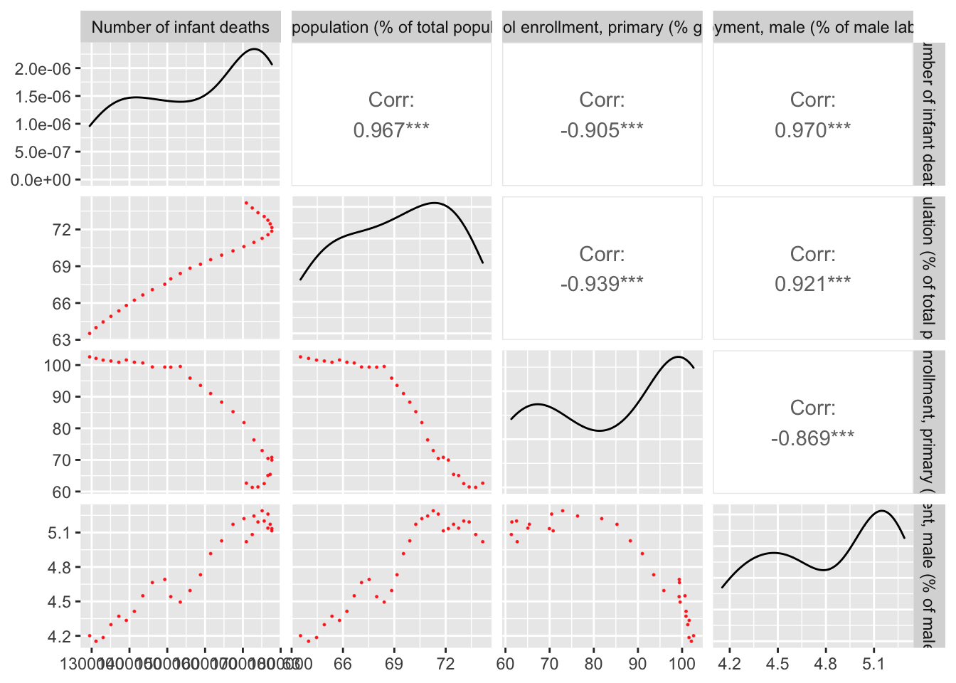
Here we can see trend emerging between Unemployment, Infant Deaths, Rural Population and School Enrollment. Some key observations:
- Unemployment and the Number of Infant Deaths has a positive, upward linear trend. This can be interpreted as there being larger number of infant deaths with rising unemployment.
How can we interpret this? Rising unemployment encompasses all professions, including medical personnel and staff. Understaffed medical facilities or untrained doctors can lead to greater occurrences of accidents and miscarriages during the process of delivery.
- Unemployment rises with a growing rural population
This observation can be supported by a growing economic trend towards technologically advanced jobs and workstreams. Rural workplaces, not financially equipped to integrate this change fall behind urban workplaces. A larger rural population with a stagnant job growth rate will result in higher unemployment levels.
- Higher school enrollment lowers unemployment
Educated individuals means a larger share of a labour force being suited for a wider range of jobs. Therefore, a higher level of education reduces unemployment.
Let’s take a more visual look at these relationships:
ggcorr(miec_mod_hipc,
method = c("everything", "pearson")) +
ggplot2::theme(legend.position = "bottom")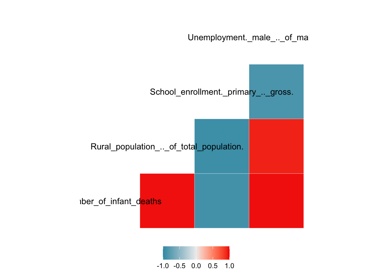 In the figure above we see that unemployment in HIPC countries is highly
correlated with rural population and infant deaths in particular, with
correlation coefficient measures nearing 1, confirmed by the upper-right half
of the scatter plot matrix above.
In the figure above we see that unemployment in HIPC countries is highly
correlated with rural population and infant deaths in particular, with
correlation coefficient measures nearing 1, confirmed by the upper-right half
of the scatter plot matrix above.
Comparing this to OECD countries:
#OECD
miec_mod_oecd<-micro_econi %>%
filter(`Country Name` == "OECD members")
miec_mod_oecd<-select(miec_mod_oecd,-c(year,
`Country Name`,
`GDP per capita (current US$)`))
ggpairs(miec_mod_oecd,
progress = F,
lower = list(continuous = wrap("points",
alpha = 0.8,
size=0.2,
colour="red")))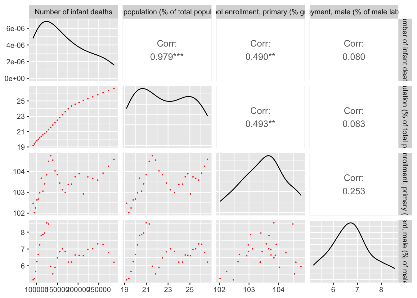 Surprisingly, different trends emerge with the same variables in an OECD
setting. Unemployment does not have strong correlations between any of the other
covariates. In fact, the only 2 variables that are hgihgly correlated are Rural
Population and Infant Deaths.
Surprisingly, different trends emerge with the same variables in an OECD
setting. Unemployment does not have strong correlations between any of the other
covariates. In fact, the only 2 variables that are hgihgly correlated are Rural
Population and Infant Deaths.
Confirming this with the correlation matrix:
ggcorr(miec_mod_oecd,
method = c("everything", "pearson")) +
ggplot2::theme(legend.position = "bottom")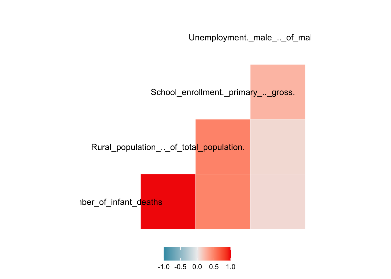 This figure agrees with the scatter plot matrix.
Given this preliminary analysis, our next objective is to use this data and build a model that can efficiently establish relationships between covariates and simultaneously predict future metrics. We start again with HIPC:
#making model for HIPC
micro_econi_hipc<-micro_econi %>%
  filter(`Country Name` == "Heavily indebted poor countries (HIPC)")
micro_econi_hipc
## # A tibble: 29 x 7
## `Number of infa… `Rural populati… `School enrollm… `Unemployment, …
## <dbl> <dbl> <dbl> <dbl>
## 1 1709223 74.2 62.7 5.02
## 2 1724841 73.8 61.3 5.08
## 3 1739922 73.4 61.4 5.19
## 4 1756412 73.1 62.5 5.20
## 5 1766214 72.8 65.1 5.14
## 6 1772358 72.5 65.4 5.17
## 7 1776749 72.2 70.0 5.13
## 8 1776527 71.9 70.8 5.11
## 9 1766385 71.6 70.5 5.26
## 10 1750964 71.3 73.0 5.29
## # … with 19 more rows, and 3 more variables: `GDP per capita (current
## # US$)` <dbl>, year <dbl>, `Country Name` <chr>par(mfrow=c(1,2))
scatter.smooth(x=micro_econi_hipc$`Rural population (% of total population)`,
y=micro_econi_hipc$`Unemployment, male (% of male labor force)`,
xlab="Rural population (% of total population)",
ylab="Unemployment, male (% of male labor force)")
scatter.smooth(x=micro_econi_hipc$`Number of infant deaths`,
y=micro_econi_hipc$`Unemployment, male (% of male labor force)`,
xlab="Number of infant deaths",
ylab="Unemployment, male (% of male labor force)") 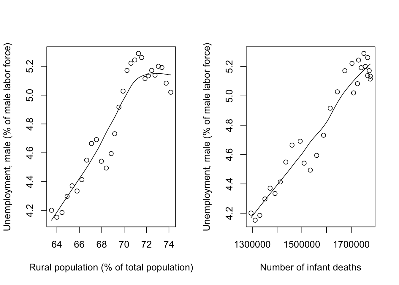 The scatter plots above relate Unemployment to Number of Infant Deaths and Rural
Population. Recall that these were the covariates which had significant
correlations to Unemployment. We can see an upward and mostly linear trend
between both sets of these variables. Therefore, a linear regression was deemed
an appropriate model.
The scatter plots above relate Unemployment to Number of Infant Deaths and Rural
Population. Recall that these were the covariates which had significant
correlations to Unemployment. We can see an upward and mostly linear trend
between both sets of these variables. Therefore, a linear regression was deemed
an appropriate model.
Our model selection strategy was guided by the previous analysis, however, we used the backward selection method to evaluate all possible models. The output for this analysis is shown:
#backward selection
micro_econi_back<-micro_econi_hipc %>%
  select(-c(year,`Country Name`))
models <- regsubsets(`Unemployment, male (% of male labor force)`~.,
                     data = micro_econi_back,
                     nvmax = 3,
                     method="backward")
summary(models)$which
## (Intercept) `Number of infant deaths`
## 1 TRUE TRUE
## 2 TRUE TRUE
## 3 TRUE TRUE
## `Rural population (% of total population)`
## 1 FALSE
## 2 FALSE
## 3 TRUE
## `School enrollment, primary (% gross)` `GDP per capita (current US$)`
## 1 FALSE FALSE
## 2 FALSE TRUE
## 3 FALSE TRUEFrom the output above, we can conclude that an adequate model has the Number of Infant Deaths as the sole covariate. We confirm this by running the two models proposed and assessing diagnostics:
micro_mod_1a<-lm(`Unemployment, male (% of male labor force)`~
                `Rural population (% of total population)` +
                 `Number of infant deaths`,
              data=micro_econi_hipc)

#final model:
micro_mod_1b<-lm(`Unemployment, male (% of male labor force)`~
                 `Number of infant deaths`,
              data=micro_econi_hipc)


#model diagnostics:
modelSummary1a <- summary(micro_mod_1a)
modelSummary1b <- summary(micro_mod_1b)
modelSummary1a
##
## Call:
## lm(formula = `Unemployment, male (% of male labor force)` ~ `Rural population (% of total population)` +
## `Number of infant deaths`, data = micro_econi_hipc)
##
## Residuals:
## Min 1Q Median 3Q Max
## -0.19778 -0.06376 0.01488 0.07499 0.14476
##
## Coefficients:
## Estimate Std. Error t value
## (Intercept) 2.470e+00 8.951e-01 2.759
## `Rural population (% of total population)` -3.040e-02 2.196e-02 -1.385
## `Number of infant deaths` 2.804e-06 4.187e-07 6.696
## Pr(>|t|)
## (Intercept) 0.0105 *
## `Rural population (% of total population)` 0.1779
## `Number of infant deaths` 4.19e-07 ***
## ---
## Signif. codes: 0 '***' 0.001 '**' 0.01 '*' 0.05 '.' 0.1 ' ' 1
##
## Residual standard error: 0.09477 on 26 degrees of freedom
## Multiple R-squared: 0.9443, Adjusted R-squared: 0.94
## F-statistic: 220.4 on 2 and 26 DF, p-value: < 2.2e-16modelSummary1b##
## Call:
## lm(formula = `Unemployment, male (% of male labor force)` ~ `Number of infant deaths`,
## data = micro_econi_hipc)
##
## Residuals:
## Min 1Q Median 3Q Max
## -0.200910 -0.066810 0.007432 0.076564 0.163667
##
## Coefficients:
## Estimate Std. Error t value Pr(>|t|)
## (Intercept) 1.253e+00 1.734e-01 7.224 9.05e-08 ***
## `Number of infant deaths` 2.243e-06 1.089e-07 20.602 < 2e-16 ***
## ---
## Signif. codes: 0 '***' 0.001 '**' 0.01 '*' 0.05 '.' 0.1 ' ' 1
##
## Residual standard error: 0.09637 on 27 degrees of freedom
## Multiple R-squared: 0.9402, Adjusted R-squared: 0.938
## F-statistic: 424.5 on 1 and 27 DF, p-value: < 2.2e-16From this output, we concluded that the model with 1 covariate (Number of Infant Deaths) along with an intercept is an appropriate model for this data. In the first model, we can see that only 1 of the covariates is significant at the 99% significance level and that the R-Squared value is approximately 0.94. Contrastingly, in the second model, we can see that both the intercept and the covariate is singificant. The R-Squared value is approxiamately identical.
There are many reasons why the Rural Population covariate, despite having a
significant correlation with Unemployment, fails to be a good predictor. One of
main reasons might be multicollinearity which is the phenomenon when one
predictor variable can be accurately predicted from others. The covariate of
Number of Infant Deaths could possibly be predicted from other covariates,
making any other variables non-significant. This also explains why our final
model has a very low p-value, indicating the significance of the model and
no presence of omitted variable bias.
Now conducting a similar regression analysis for OECD members:
#Model for OCED
micro_econi_oecd<-micro_econi %>%
  filter(`Country Name` == "OECD members")
micro_econi_oecd
## # A tibble: 29 x 7
## `Number of infa… `Rural populati… `School enrollm… `Unemployment, …
## <dbl> <dbl> <dbl> <dbl>
## 1 286588 26.6 105. 6.22
## 2 273373 26.3 104. 6.79
## 3 260376 26.1 104. 7.28
## 4 247657 25.8 104. 7.30
## 5 235410 25.5 104. 7.01
## 6 223728 25.3 104. 6.97
## 7 212692 25.0 103. 6.60
## 8 202538 24.8 104. 6.63
## 9 193113 24.6 104. 6.64
## 10 184356 24.3 103. 6.22
## # … with 19 more rows, and 3 more variables: `GDP per capita (current
## # US$)` <dbl>, year <dbl>, `Country Name` <chr>par(mfrow=c(1,3))
scatter.smooth(x=micro_econi_oecd$`School enrollment, primary (% gross)`,
y=micro_econi_hipc$`Unemployment, male (% of male labor force)`,
xlab="School enrollment, primary (% gross)",
ylab="Unemployment, male (% of male labor force)")
scatter.smooth(x=micro_econi_oecd$`Rural population (% of total population)`,
y=micro_econi_hipc$`Unemployment, male (% of male labor force)`,
xlab="Rural population (% of total population)",
ylab="Unemployment, male (% of male labor force)")
scatter.smooth(x=micro_econi_oecd$`Number of infant deaths`,
y=micro_econi_hipc$`Unemployment, male (% of male labor force)`,
xlab="Number of infant deaths",
ylab="Unemployment, male (% of male labor force)") 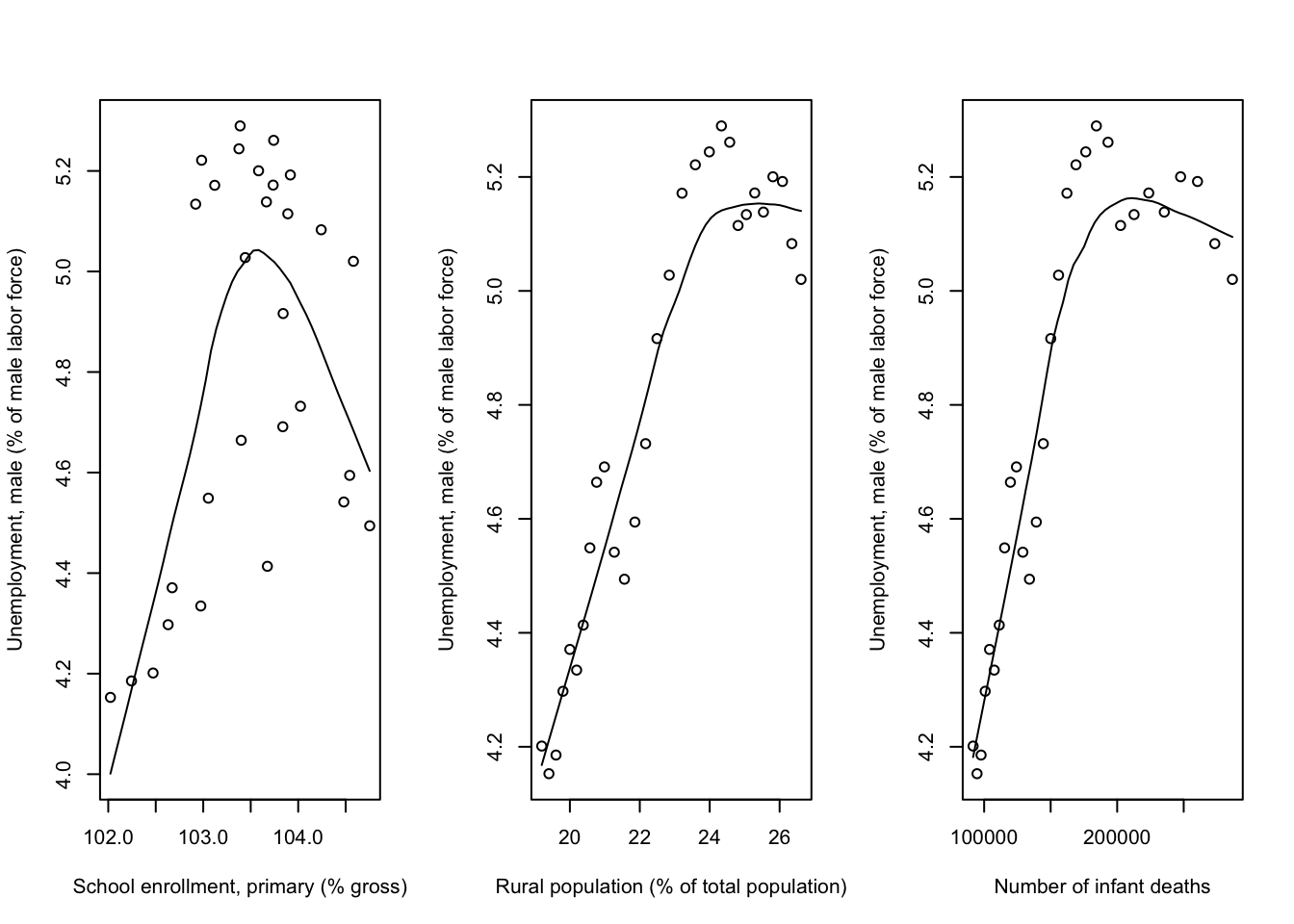 From the scatter plots above, we see that there is a roughly linear trend for
Unemployment with Rural Population and Infant Deaths. However, there is no clear
between Unemployment and School Enrollment. This observation, combined with our
preliminary analysis which indicated low correlation levels between Unemployment
and all other covariates, suggests that Unemployment may not be the most
appropritate response variable. In fact, looking back to the correlation matrix,
we see that Rural Population and Infant Deaths had the highest correlation.
From the scatter plots above, we see that there is a roughly linear trend for
Unemployment with Rural Population and Infant Deaths. However, there is no clear
between Unemployment and School Enrollment. This observation, combined with our
preliminary analysis which indicated low correlation levels between Unemployment
and all other covariates, suggests that Unemployment may not be the most
appropritate response variable. In fact, looking back to the correlation matrix,
we see that Rural Population and Infant Deaths had the highest correlation.
Therefore, we decided to look at the relationship between the two correlated variables:
scatter.smooth(x=micro_econi_oecd$`Rural population (% of total population)`,
y=micro_econi_oecd$`Number of infant deaths`,
xlab="Rural population (% of total population)",
ylab="Number of infant deaths")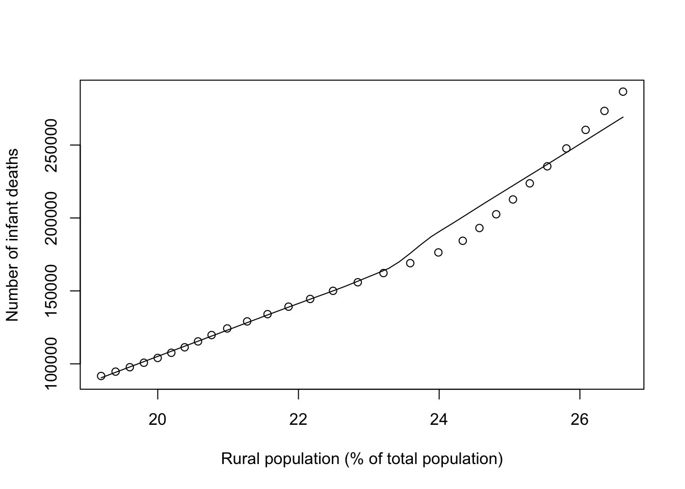 Unsurprisingly, an almost perfectly linear trend emerges.
This finding encouraged us to pursue a model with Infant Deaths as the response variable. However, before we discard Unemployment as the response variable, we were eager to study if the approxiamately linear trends between that and Rural Population and Infant Deaths would be captured by a model.
#backward selection
micro_econi_back2<-micro_econi_oecd %>%
  select(-c(year,`Country Name`))
models2 <- regsubsets(`Unemployment, male (% of male labor force)`~.,
                      data = micro_econi_back2,
                      nvmax = 3,
                      method="backward")
summary(models2)$which
## (Intercept) `Number of infant deaths`
## 1 TRUE FALSE
## 2 TRUE FALSE
## 3 TRUE FALSE
## `Rural population (% of total population)`
## 1 FALSE
## 2 FALSE
## 3 TRUE
## `School enrollment, primary (% gross)` `GDP per capita (current US$)`
## 1 TRUE FALSE
## 2 TRUE TRUE
## 3 TRUE TRUEmicro_mod_2<-lm(`Unemployment, male (% of male labor force)`~
`School enrollment, primary (% gross)`,
data=micro_econi_oecd)
modelSummary <- summary(micro_mod_2)
modelSummary##
## Call:
## lm(formula = `Unemployment, male (% of male labor force)` ~ `School enrollment, primary (% gross)`,
## data = micro_econi_oecd)
##
## Residuals:
## Min 1Q Median 3Q Max
## -1.53916 -0.48295 0.04195 0.40863 1.70238
##
## Coefficients:
## Estimate Std. Error t value Pr(>|t|)
## (Intercept) -25.4803 23.6736 -1.076 0.291
## `School enrollment, primary (% gross)` 0.3113 0.2287 1.361 0.185
##
## Residual standard error: 0.8518 on 27 degrees of freedom
## Multiple R-squared: 0.0642, Adjusted R-squared: 0.02954
## F-statistic: 1.852 on 1 and 27 DF, p-value: 0.1848After conducting backward selection, we found that a model with School Enrollment as the sole predictor was recommended. However, this model has a high element of bias present. Firstly, none of the covariates (including the intercept) are significant. This suggests a variable bias is present. Additionally, the p-value for the model is 0.1848, higher than any acceptable significance levels. The R-Squared supports this pattern, with an unusually low value appearing.
Therefore, we decided to pursue our modified model for OECD members.
models3 <- regsubsets(`Number of infant deaths`~.,
                      data = micro_econi_back2,
                      nvmax = 3,
                      method="backward")
summary(models3)$which
## (Intercept) `Rural population (% of total population)`
## 1 TRUE TRUE
## 2 TRUE TRUE
## 3 TRUE TRUE
## `School enrollment, primary (% gross)`
## 1 FALSE
## 2 FALSE
## 3 TRUE
## `Unemployment, male (% of male labor force)` `GDP per capita (current US$)`
## 1 FALSE FALSE
## 2 FALSE TRUE
## 3 FALSE TRUEWe performed backward selection once again to find that the intercept and Rural Population were chosen as the covariates for a model with Infant Deaths as the response variable.
#final model:
micro_mod_2b<-lm(`Number of infant deaths`~
                 `Rural population (% of total population)`,
              data=micro_econi_oecd)

#model diagnostics:
modelSummary2b <- summary(micro_mod_2b)
modelSummary2b
##
## Call:
## lm(formula = `Number of infant deaths` ~ `Rural population (% of total population)`,
## data = micro_econi_oecd)
##
## Residuals:
## Min 1Q Median 3Q Max
## -18353 -8662 1456 6233 29519
##
## Coefficients:
## Estimate Std. Error t value
## (Intercept) -378039.3 21821.2 -17.32
## `Rural population (% of total population)` 23864.5 956.2 24.96
## Pr(>|t|)
## (Intercept) 3.75e-16 ***
## `Rural population (% of total population)` < 2e-16 ***
## ---
## Signif. codes: 0 '***' 0.001 '**' 0.01 '*' 0.05 '.' 0.1 ' ' 1
##
## Residual standard error: 12060 on 27 degrees of freedom
## Multiple R-squared: 0.9585, Adjusted R-squared: 0.9569
## F-statistic: 622.9 on 1 and 27 DF, p-value: < 2.2e-16As expected, the model has significant covariates, along with a significant p-value.
Conclusions From Microeconomic Analysis:
From our analysis of microeconomic variables on the two sets of countries, we have found many differences in the economic workings of both countries.
While analysing HIPC economies, we saw how unemployment, a vital measure in micro and macro economic analyses, was determined by an number of covariates, namely the number of infant deaths (mortality rate) and the percentage of rural population (out of total population). When we performed regression analysis however, we found that only the number of infant deaths was a good predictor for unemployment.
At a microeconomic level, this paints a grim picture. It suggests that mortality rates are directly correlated with the level of unemployment in poorer countries. Unemployment measures, which encompass all work streams, include the medical profession. Therefore, large unemployment in the medical sector, according to our model, causes a lack of educated personnel and pediatricians. In a healthy environment, such individuals are vital for the wellbeing of an infant. A lack of sufficient medical care and educated personnel lead to a higher mortality rate. Additionally, widespread unemployment also indicates the lack of ability of parents and guardians to provide a safe environment for an infant. Therefore, unemployment and infant mortality rates portray a correlated relationship. This is supported by our model which indicates a positive coefficient for the infant death covariate. An increase in infant deaths, caused by higher levels of unemployment, lead to increased unemployment, which in turn causes higher infant mortality rates.
In OECD countries, the effect of microeconomic factors such as infant mortality rates and school enrollment levels are not directly correlated to unemployment. There are many reasons why this may be true. One of the reasons is due to a large number of external factors and measures which cause unemployment in a developed setting. These factors do not exist in a developing environment. An example of such a factor is monetary policy changes made by the central bank. These changes directly impact unemployment levels and are felt to a lesser extent in a smaller economy with a smaller central bank.
Shifting our analysis to account for this change in environment, our analysis found that in developed economies the infant mortality rate is directly correlated with the proportion of rural population. In a developed environment, urban population has access to a large number of childcare options, which may not always be available to the rural population. This, in addition to the fact that statistically the majority of rural population is provided sub-optimal educational resource, a lack of knowledge and ability leads to a greater number of infant deaths.